Geophysical curiosity 66 & 67
Rock-physics relationships are different from what you thought.
Another interesting publication in “The leading Edge” of 2016 by Michelle Thomas et al., on the incorrect relationships used by many when dealing with inverted elastic parameters. Namely, we should not assume that the original rock-physics relationship applies to inverted properties This was demonstrated using one of the many linearized AVO expressions.
For
example, calculating the coefficients to convert the inverted (estimated)
intercept (Iest) and gradient (Gest), inverted using the Goodway
linearisation based on VP/VS=2: 
results in RPest=1.05Iest and RSest=1.28Iest-0.5Gest,whereas the true rock-physics relationship is RP=I and RS=0.5I-0.5G.
The idea of using the true rock-physics weights, to estimate elastic reflectivity based on inversion results is part of the “holy grail” of seismic interpretation but above is one of the many examples of where it is in error.
In the context of extended elastic impedance (EEI) it should be noted that also for EEI the relationships between the inverted rock properties can differ from the true rock property relationships, depending on which AVO equation was used.
AVO revisited
Sometimes it is a good idea to go back to older publications, which was the case looking back at the May issue of the “The Leading Edge” of 2016 on AVO inversion. In this issue two inversion approaches were compared : the frequentist and the statistical inversion. The frequentist considers the subsurface properties fixed but unknown, whereas the Bayesian statistical inversion characterizes our prior understanding of the “fixed” but unknown subsurface properties.
In the frequentist approach the forward model is regularized to avoid the model null space, the parameter space that does not influence the seismic, but destabilize the inversion. In the Bayesian method it is the prior information that stabilizes the inversion.
Two interesting alternatives in the Bayesian method exists: two-step in which first the elastic parameters are estimated followed using a rock-physics model to find the rock parameters and the one-step in which the rock parameters are directly estimated. Also, the posterior probability distribution, which is the answer, can be sampled to investigate whether the distribution is a composite (Gaussian) mixture model.
If the prior distribution is a single (Gaussian) model, the maximum a posteriori solution (MAP) is the same as the frequentist solution.
Fresnel zone
The
question is: “Do I always need to honour the “Nyquist” requirement when
sampling data?” Sampling a time series, it is indeed the case, but sampling in
space is a different question. Let us
look at seismic reflection data. The recorded
energy consist of so-called Frauenhofen rings of which in seisnmic only the
dominant first order one is considered. For 2D with a source
receiver offset X the Fresnel radius equals 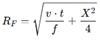 For zero offset the Fresnel radius is determined by the additional
distance λ/4 from the source to scattering point. This leads in 2D to a contributing circle. For
an offset X it results in an ellipse with the longer axis in the
source-receiver direction. The
consequence is that the reflected energy contains information on the interface
over a larger inline area and thus the spatial interval can be taken larger
than required by the Nyquist criteria, without any loss of information. The
fresnelzones for a single source and receivers arond it are nicely shown in the
displays below (Goodway et al., FB2024,N9)
For zero offset the Fresnel radius is determined by the additional
distance λ/4 from the source to scattering point. This leads in 2D to a contributing circle. For
an offset X it results in an ellipse with the longer axis in the
source-receiver direction. The
consequence is that the reflected energy contains information on the interface
over a larger inline area and thus the spatial interval can be taken larger
than required by the Nyquist criteria, without any loss of information. The
fresnelzones for a single source and receivers arond it are nicely shown in the
displays below (Goodway et al., FB2024,N9)
Whatever happened to
super-critical reflections?
Preparing a course on AVO and Inversion, I became interested in the use of super-critical reflections. These occur in case the velocity across an interface increases and are especially prominent in case of carbonates, salt and basalt layers, where the P-wave velocity is often much larger than the overburden. I looked in the geophysical literature for relevant publications and found some, but not many. In the publications, it was claimed that super-critical reflections could be beneficial for reservoir characterisation even with signal-to-noise levels as low as two. Although most investigations were limited to isotropic media and incident plane-waves, there is no reason it could not be extended to more realistic media. For example, I wonder whether super-critical reflections have ever been used in Full Waveform Inversion or in a Machine Learning context. My question to the reader of this note: Can you inform me of interesting publications that make use of super-critical reflections for reservoir characterisation?
Jaap Mondt, website: www.breakawayleaning.nl, email: j.c.mondt@planet.nl
Appendix: Investigations in Geophysics, N8 (Castagna & Backus). P5-6
After Richards,T.C. Geophysics 1961, P277-297
1. P-wave local maxima may occur at normal incidence, first critical angle, and possibly near the S-wave critical angle.
2. The change of the reflection coefficient with angle is small at low angles.
3. The first critical angle is given by sinθc1=VP1/VP2. When VP1>VS2 there is no critical angle
4. The second critical angle is given by sinθc2=VP1/VS2. Beyond this critical angle there is no transmitted S-wave. When VP1>VS2 there is no second critical angle and converted S-waves will be transmitted at all angles below 90°
5. S-wave conversions, both reflected and transmitted are strongest between first critical angle and grazing incidence.
6. The reflection coefficient becomes complex beyond the critical angle.
7. The reflection coefficient and transmission coefficient are frequency independent.
8. The reflection coefficient from above is not equal to the one from below (asymmetrical).
9. Spherical waves exhibit frequency dependent reflection coefficients, and its maximum occurs beyond the critical incidence
No need for ultralong
offsets anymore?
In a series of interesting articles, it was discussed whether Full Waveform Inversion (FWI) and Least-Squares Reverse Time Migration (LSRTM) could be combined as both update model parameters using the difference between modelled and observed data. And indeed, a workflow was proposed in which in an iterating sequence both were combined. In addition, the wave equation, normally involving the density as a parameter, was reformulated in terms of velocity and vector reflectivity. The vector reflectivity was related to the acoustic impedance image calculated by RTM using a velocity model from FWI in the sequence. Experiments with synthetic and real data showed the correctness of the approach, with a benefit of reducing the cycle time as hardly any preprocessing is needed. In a later publication it was demonstrated that the method could be applied pre-stack, allowing AVA analysis. But here comes probably the main advantage: ultra long offsets are no longer needed.
Ref: Chemingui et al, First Break July 2024
A breakthrough with
Invertible Neural Networks?
In geophysics we often need to determine subsurface model parameters from a set of measurements. Usually, the forward process from parameter- to measurement-space is reasonably well-defined, whereas the inverse problem is ambiguous: multiple parameter sets can result in the same measurement. To fully characterize this ambiguity, the full posterior parameter distribution, conditioned on an observed measurement, must be determined. Not only the best value but also its uncertainty (standard deviation or better the full posterior distribution) must be determined. Traditionally this is done using Bayesian inversion, demanding prohibitive compute time, however.
Suitable for this task are Invertible Neural Networks (INNs). Unlike classical neural networks, which attempt to solve the ambiguous inverse problem directly, INNs focus on learning the forward process, using additional latent output variable distributions z to capture the information otherwise lost. Due to invertibility, a model (extended with latent model parameter distributions ε) of the corresponding inverse process is learned implicitly.
Given a specific measurement and the distribution of the latent variables, the inverse pass of the INN provides the full posterior parameter space. INNs are capable of also finding multi-modalities in parameter space, uncover parameter correlations, and identify unrecoverable parameters (ε).
INNs are characterized by: (I) The mapping from inputs to outputs is bijective, i.e. its inverse exists, (ii) both forward and inverse mapping are efficiently computable, and (iii) allow explicit computation of model posterior probability distributions. Networks that are invertible by construction offer a unique opportunity: We can train them on the well-understood forward process x → y and get the inverse [y, z] → [x, ε] for free by running them backwards.
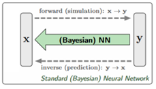
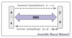
Abstract comparison of standard Bayesian (left) and INN (right). The Bayesian direct approach requires a discriminative, supervised loss (SL) term between predicted and true x, causing problems when y → x is ambiguous. INN uses a supervised loss only for the well-defined forward process x → y. Generated x is required to follow the prior p(x) by an unsupervised loss (USL), while the latent variables z is made to follow a Gaussian distribution (a choice), also by an unsupervised loss.
To counteract the inherent information loss of the forward process, due to approximate physics, we introduce additional latent output variables z, which capture the information about x that is not contained in y. Thus, INN learns to associate hidden parameter values x with unique pairs [y, z] of measurements and latent variables (z, ε). Forward training optimizes the mapping [y, z] = f (x) and implicitly determines its inverse x = f −1(y, z) = g (y, z). Additionally, we make sure that the pdf p(z) of the latent variables is shaped as a Gaussian distribution (a choice). Thus, the INN represents the desired posterior p(x|y) by a deterministic function x = g(y, z) that transforms (“pushes”) the known distribution p(z) to x-space, conditional on y. Compared to standard Bayesian approaches, INNs circumvent a fundamental difficulty of learning inverse problems. If the loss does not match the complicated (e.g. multi- modal) shape of the posterior, learning will converge to incorrect or misleading solutions. Since the forward process is usually much simpler and better understood, forward training diminishes this difficulty. Specifically, we make the following contributions:
• We show that the full posterior of an inverse problem can be estimated with invertible networks, both theoretically in the asymptotic limit of zero loss.
• The architectural restrictions imposed by invertibility do not seem to have detrimental effects on our network’s representational power.
• While forward training is sufficient in the asymptotic limit, we find that a combination with unsupervised backward training improves results on finite training sets.
• In geophysical applications, our approach to learning the posterior pdf compares favourably to approximate Bayesian computation and conditional Variational Auto-Encoders (VAE). This enables identifying unrecoverable parameters, parameter correlations and multimodalities.
Ref: Ardizzone et al., arXiv:1808.04730v3
Can geophysics help improving reservoir simulation?
Yes, indeed it can and in a relatively inexpensive way by using time-lapse measurements of gravity and subsidence. In a recent publication, Equinor shows that seafloor gravity and pressure measurements have sufficient accuracy to measure the gravity changes due to production of a condensate field at a seafloor depth of about 2500m. Thirty-one permanent platforms were installed above the field, at distances corresponding the depth of the reservoir. Given the quiet seafloor environment, the measurements were accurate in the order of one micro-Gal and a few millimetres.
The time-lapse recordings showed that the reservoir simulation model should be updated to improve the match with the observed gravity data. This has significant consequences for the future production strategy of the field.
The principle of reciprocity
Q1: The principle of reciprocity tells us that when source
and receive locations are interchanged, the same seismic responses should be
obtained. At first sight, this suggest that by using it we do not add any new
information. Hence, why do we still get an improvement in the final image? Is
it because we double the number of traces in the migration input?
Q2: When I compare fig a and b, I notice a difference in seismic bandwidth. Fig 9b seems to have a lower resolution. If so, what is the reason?
VTI RTM End-on shot gathers VTI RTM Interpolated PSS shot gathers

A1: Regarding the principle of reciprocity, you are correct that it suggests that when we interchange source and receiver locations, we should obtain the same seismic responses. However, even though this may not seem to add new information at first glance, there are reasons why we still see improvements in the final image. One key factor is that by using reciprocity, we effectively double the number of traces in the migration input. This increase in the number of traces can lead to improvements in the signal-to-noise ratio (S/N) and, consequently, result in a better final image. Similarly, when we interpolate, we are also increasing the number of input traces, which can enhance the S/N ratio further.
A2: The reason for this difference may be multifaceted and would require a more detailed analysis. It could be related to the interpolation process or other factors during migration.
References: Liang
et al., Geophysics 2017, N4
What happened with spectral bandwidth extension?
As seismic data is bandlimited due to source limitation and attenuation of the high frequencies during propagation, the resolution of seismic data is limited. Conventionally defined as a quarter of the dominant wavelength. Various methods exist to extend the seismic spectrum beyond the Nyquist frequency: phase acceleration, loop re-convolution and harmonic extrapolation:
Phase acceleration
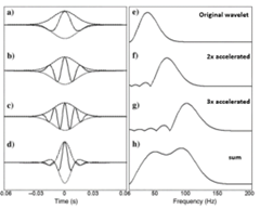
The analytic signal is the complex signal with the original signal as the real part and the Hilbert transform as the imaginary part. Phase acceleration uses the instantaneous frequency (time derivative of the instantaneous phase). Then the phase and thus the frequency is shifted by multiplication. In the example that is done twice, and the resulting analytic signals are added, resulting in an increased bandwidth.
Loop re-convolution
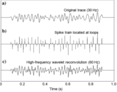
In loop re-convolution spikes are positioned at loop minima and maxima and the spike train is then convolved with a higher frequency wavelet. This results in a higher frequency, broader bandwidth seismic trace.
But do these procedures lead to higher resolution?
Let us look at a third method: Harmonic extrapolation.
If we can assume that the earth conforms to a blocky impedance structure, then the frequency spectrum can be seen as a superposition of sinusoidal layer frequency responses and each layer frequency can be extrapolated using a basis-pursuit method. Better?
Results for a wedge model:
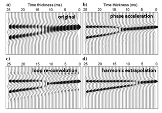
Both phase acceleration and loop re-convolution lead to sharper interfaces, but not to a better thickness resolution. Only the harmonic extrapolation increases the resolution, moving the wedge point from 17ms to 7ms.
Application to real seismic using well synthetic comparisons.
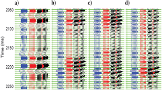
well-log synthetic (blue), composite
(summed) seismic (red), seismic around well (black)
a) the original wavelet (10-80-120-130Hz (0.96), double frequency versions of b) phase acceleration (0.20), c) loop re-convolution (0.45), d) harmonic extrapolation (0.72)
The correlations (0.20, 0.45, 0.72) with the well synthetic showed the superior result of harmonic extrapolation.
One main advantage of harmonic extrapolation is when filtered back to the original bandwidth, the same seismic trace results, which is not the case for the other methods.
Reference: Liang et al., Geophysics 2017, N4
How Geophysics fuels the
Energy Transition
Geothermal energy plays a significant role in the energy transmission. The method is based on injecting cold and extracting hot water from a hot layer in the Earth. For this the rock layer between injector and extractor should have sufficient porosity and permeability. But how to predict these rock properties between wells?
Here
geophysics will be the enabler. In a publication published in The Leading Edge,
a successful combination of Machine Learning and Rock-physics was used to
predict porosity and permeability in between wells. A Deep Neural Network (DNN)
was trained to predict from seismic traces the porosity and permeability of a
geothermal reservoir layer. The rock-physics model was used to connect rock
properties with elastic properties. The limited training data (only 4 logged
wells) was augmented. Also, realistic noise was added to the synthetic traces
to make them appear like real seismic. A second DNN was used to predict from
seismic the clay content, so that effective porosity could be calculated. The
permeability was predicted from the effective porosity using a statistical
relationship derived from core samples.
The network was applied to seismic of the Dogger formation in the Paris basin to predict additional geothermal drilling sites
See the video on https://breakawaylearning.nl
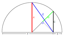
Arithmetic: A=(a+b)/2
Geometric: G=√ab
Root mean square: Q=√(a2+b2)/2
Harmonic 1/[(1/a+1/b)/2]-2ab/(a+b)
if a≠b: H<G<G<Q
if a=b: H=G=A=Q
if either a or b is zero: A=a/2, Q=√2a, G=0, H=0
if a=0=b: H not defined
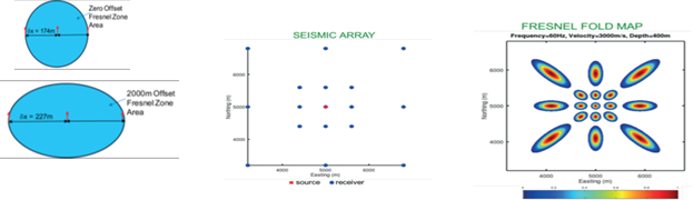
Data and Model Resolution
Suppose we have found a generalized inverse that
solves the inverse problem Gm=d, with N data and M model parameters, yielding
an estimate of the model parameters mest=G-gd. Substituting
our estimate in the equation GM=d yields:
dpre=Gmest=G[G-gdobs]=[GG-g]dobs=Ndobs
The NxN square matrix N=GG-g is the data
resolution matrix
Suppose there is a true model mtrue that
satisfies Gmtrue=dobs. Substituting this in the
expression for the estimated model mest=G-gdobs
yields:
mest=G-gdobs=G-g[Gmtrue]=[G-gG]mtrue=Rmtrue
The MxM square matrix R=G-gG is the model
resolution matrix. If R is not the identity matrix, then the estimated model
parameters are weighted averages of the true model parameters.
Overdetermined system: N>M then the least-squares
inverse equals:
G-g=[GTG]-1GT
N=GG-g=G[GTG]-1GT
R=G-gG=[GTG]-1GTG=I
Underdetermined system: N<M then the
least-squares inverse equals:
G-g=GT[GGT]-1
N=GG-g=GGT[GGT]-1=I
R=G-gG=GT[GGT]-1G
Ref: W. Menke Geophysical Data Analysis: Discrete Inverse Theory
De-risking CO2 storage
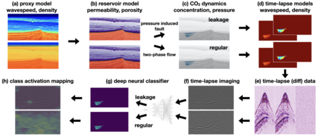
A synthetic data set based
on a North Sea (Blunt) sandstone reservoir and a seal (Rot Halite) was created
(a). Using a rock physics model, the reservoir porosity and permeability were
calculated based on the velocity and density (b). As a result of the injection
pressure, fractures in the seal were created, leading to two model sets: with leakage
and without leakage (c,d)) Shot gathers (e) and time-lapse sections (f) were
generated for the two different sets of models.
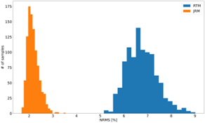
The usual method for evaluating the effectiveness of time-lapse seismic is by calculating the Normalised-Mean-Root-Square metric (NMRS). For the synthetic data the NRMS errors for the Joint and Separate inversions were 2.30% and 8.48%, respectively, which shows that joint inversion is preferred. Also the spread for the joint inversion is much lower.
Then a highly sensitive Deep Neural Classifier (Vision Transformer, ViT) was trained (g) to classify seismic into leakage and no leakage (regular). The results were posted on the sections (h). The trained network was applied to classification of 206 unseen test instances, with the following results:
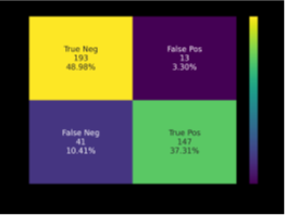
Predictions:
TP=True Positive, FP=False Positive, TN=True negative, FN=False Negative, Precision=TP/(TP+FP
)= 91.8%, Recall=TP/(TP+FN) ==43.2%, F1=TP/(TP+½(FN+FP))
=58.8%
Conclusion: Using Deep Neural Networks yields a significant improvement in NMRS values, without requiring replication of the baseline survey. While the classification results are excellent, there are still False Negatives (FN). This might be acceptable as the decision to stop injection of CO2 should also be based on other information, such as pressure drop at the well head.
The method will be discussed in my courses (www.breakawaylearning.nl).
Ref: Ziyi Yin, Huseyin Tuna Erdinc, Abhinav Prakash Gahlot, Mathias Louboutin, Felix J. Herrmann, arXiv:2211.03527v1
Wasserstein or Optimal Transport Metric
Intuition and connection to optimal transport
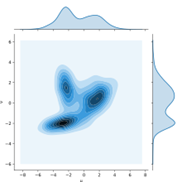
Two one-dimensional distributions μ and ν, plotted on the x and y axes, and one possible joint distribution that defines a transport plan between them. The joint distribution/transport plan is not unique. One way to understand the above definition is to consider the optimal transport problem. That is, for a distribution of mass μ(x) on a space X , we wish to transport the mass in such a way that it is transformed into the distribution ν(x) on the same space; transforming the 'pile of earth' μ to the pile ν . This problem only makes sense if the pile to be created has the same mass as the pile to be moved; therefore, without loss of generality assume that μ and ν are probability distributions containing a total mass of 1. Assume also that there is given some cost function: c (x,y) ≥ 0.that gives the cost of transporting a unit mass from the point x to the point y. A transport plan to move μ into ν can be described by a function γ(x,y) which gives the amount of mass to move from x to y. You can imagine the task as the need to move a pile of earth of shape μ to the hole in the ground of shape ν such that at the end, both the pile of earth and the hole in the ground completely vanish. For this plan to be meaningful, it must satisfy the following properties:
∫γ(x,y)dy=μ(x) (the amount of earth moved out of point x needs to equal the amount that was there to begin with)
∫γ(x,y)dx=ν(y) (the amount of earth moved into point y needs to equal the depth of the hole that was there at the beginning)
That is, that the total mass moved out of an infinitesimal region around x must be equal to μ(x)dx and the total mass moved into a region around y must be ν(y)dy. This is equivalent to the requirement that γ be a joint probability function distribution with marginals μ and ν. Thus, the infinitesimal mass transported from x to y is γ(x,y)dxdy, and the cost of moving is c(x,y).γ(x,y)dxdy , following the definition of the cost function. Therefore, the total cost of a transport plan γ is:
∬c(x,y)γ(x,y)dxdy = ∫c(x,y)dγ(x,y)
The plan γ is not unique; the optimal transport plan is the plan with the minimal cost out of all possible transport plans. As mentioned, the requirement for a plan to be valid is that it is a joint distribution with marginals μ and ν; letting Γ denote the set of all such measures as in the first section, the cost of the optimal plan is:
C = inf γ ∈ Γ(μ,ν)∫c(x,y)dγ(x,y)
If the cost of a move is simply the distance between the two points, then the optimal cost is identical to the definition of the Wasserstein-1 distance.
The Wasserstein Generative Adversarial Network (WGAN) is a variant of Generative Adversarial Network (GAN) that aims to improve the stability of learning, get rid of problems like mode collapse, and provide meaningful learning curves useful for debugging and hyperparameter searches". Compared with the original GAN discriminator, the Wasserstein GAN discriminator provides a better learning signal to the generator. This allows the training to be more stable when generator is learning distributions in extremely high dimensional spaces.
Wasserstein distance
The point of the discriminator is as a critic to provide feedback for the generator, about "how far it is from perfection", where "far" is defined as Jensen–Shannon divergence*. Naturally, this brings the possibility of using a different criterion of farness. There are many divergences to choose from, such as the f-divergence family, which would give the f-GAN.The Wasserstein GAN is obtained by using the Wasserstein metric, which satisfies a "dual representation theorem" that renders it highly efficient to compute:*In probability theory and statistics, the Jensen-Shannon divergence is a method of measuring the similarity between two probability distributions.
Societal Concerns with Hydraulic Fracturing
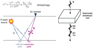
In an interesting publication in First Break 2023, N1, Tom Davis from Colorado School of Mines, shows that multi-component seismic monitoring of geo-mechanical changes reveal whether the overburden of an induced fractured reservoir is influenced by increased stress from the fracturing pressure in the reservoir or by propagation of fractures from the reservoir into the overburden. This could be observed from the travel-time changes of the fast and slow shear wave reflections of the top reservoir. Increased stress results in a decrease in the PS travel time, upward propagating fractures to an increase in travel time for the slow PS component (polarized normal to the fractures). Especially the propagation of fractures into the overburden needs monitoring in view of societal concerns with hydraulic fracturing.
A New Business Model
Dropout is one of the most popular regularization techniques for deep neural networks. It has proven to be highly successful: many state-of-the-art neural networks use dropout.
It is a simple algorithm: at every training step, every neuron (including the input, neurons, but always excluding the output neurons) has a probability p of being temporarily "dropped out”, meaning it will be entirely ignored during this training step, but it may be active during the next step. The hyperparameter p is called the dropout rate, and it is typically set between 10% and 50%, closer to 20%-30% in recurrent neural nets, and closer to 40%-50% in convolutional neural networks. After training, neurons do not get dropped anymore. It is surprising at first that this destructive technique works at all.
An analogy is the human brain. We know that when part of the brain neurons are damaged by an accident or stroke, then other parts of the brain take over the functions of the damaged part, making the brain a robust network.
Let us translate this into a business model. Would a company perform better if 10% of its employees, randomly chosen, were told every month to take vacation the next month? Most likely, it would! The company would be forced to adapt its organization; it could no longer rely on any single person to perform any critical task, so this expertise would have to be spread across several people. Employees would have to learn to cooperate with many of their co-workers, not just a handful of them. The company would become much more resilient. If one person quits; it would not have much of an impact.
It could work for companies, but it certainly does for a neural network. The network ends up being less sensitive to changes in the input, as the final network is in principle the combination of many trained networks. In the end we have a much more robust network that generalizes much better.
Adapted from “Hands-on Machine Learning with Scikit-Learn, Keras & TensorFlow, by Aurélien Géron
Multi-physics
Multi-physics is the way forward. It means that
a combination of complimentary datasets are used to get a full “picture” of the properties of
the subsurface.
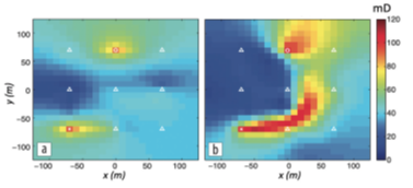
A synthetic model example (Liang et al, Geophysics 2016, N5)
is shown below where the permeability was first recovered from the inversion
of production data alone (a) and later with multi-physics inversion of
seismic, time-lapse electromagnetic and production data. The latter resulted in a much more accurate permeabilty map.
Referring to my video “You ain’t seen nothing yet “, I see a tremendous opportunity using multi-physics in combination with Machine Learning, incorporating rock-physics models.
Trans Dimensional Seismic Inversion
In inverse problems the number of model parameters is assumed to be a known quantity, and we only estimate the parameter values. However, treating the number of parameters as fixed can either lead to underfitting if the number of parameters is chosen too few or overfitting in case of too many parameters. This is, for example, the case if the number of layers for which the elastic quantities Vp, Vs and ρ are to be determined is also unknown. It is crucial to determine the exact model parametrization that is consistent with the resolving power of the data. Hence, it is sensible to make the number of model parameters part of the unknowns to be solved.
The method used to solve this issue is called Reversible Jump Hamiltonian Monte Carlo (RJHMC).
In the referenced publication AVA inversion for a horizontal stack of k+1 homogeneous layers separated by k plane interfaces with a half space below. The unknown parameters are the k P-, S-wave velocities and densities and k, the number of layers. As density was the main aim of the inversion, the full Zoeppritz equation was used.
Ref: Biswas et al., TLE 2022, N8 & Sen and Biswas, Geophysics, 2017, N3
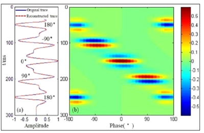
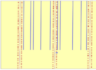
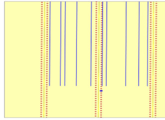
Short time-window trace to time-frequency transform can be done in many ways: among others Discrete Fourier Transform, Continuous Wavelet Transform, Inversion based and Spectral decomposition. Amplitude frequency gathers are easy to interpret, but Phase frequency gathers are very difficult to make sense out of it.
A phase decomposition expresses the amplitude of a trace as a function of time and phase. A phase gather shows the amplitude and phase information simultaneously.
In the phase decomposition plot we see distinct concentrations centred around certain phases:
-180, -90, 0, +90, +180.
We can sum the energy at -90 and +90 degrees, which is call odd phase component, or at 0 and 180 degrees, called even phase component. Summing over phase returns the original trace
Volume of Influence
When sampling data, we usually follow the Nyquist sampling theory, where we make sure that we take 2 samples for the shortest wavelength or period so that we avoid aliasing.
However, there are other ways of looking at it.
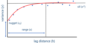
1. Using a variogram
It is well known, that in relation to space, so-called variograms are used. They show how with distance the variance between data increases and levels off. The sampling distance can be chosen based on a variance value, for example half the variogram range.
2. Using volume of influence
Consider the distance over which a physical property influences a measurement. This can be derived from physics. For example, the influence of a point mass is described by Newton’s law: F=Gm1m2/r2, hence the sphere of influence is described by 1/r-2 or for a magnetic dipole by 1/r-3. Although in principle the volume of influence is infinite, in view of noise we can limit the range of influence for a specified noise level. This results in a so-called volume of influence or investigation. This volume can be included in our requirements for sampling. See graph: r=4 for gravity, r=0.8 for a magnetic dipole.
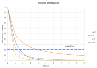
These different criteria lead to different sampling strategies. The trade-off is now between getting all the details, called a 100% characterization probability, or making sure we get the correct estimate of the presence with a lower characterization probability. Accepting a lower value will allow a coarser and less expensive sampling strategy.
Geophysical curiosity 45
Geophysical curiosity 44
Is the locus of a travel-time tAB
in (x-t) the same as in (x-z)?
We often read about an elliptical locus of equal travel time with
an offset acquisition, but do we mean in the space domain or in the space
recording time domain? Are they in both domains elliptical or not? Let us see.
In x-z
The travel time tAB= (A+B)/V= [SQRT((x+x0)2+z2)
+ SQRT((x-x0)2+z2)]
which can be written as 4x2x02-V2tAB2x2-V2tc2z2=-V4tc4/4+V2tc2x02,
which is the standard form of an ellipse: x2/a2+z2/b2=1,
with a=-Vtc/2 and b=SQRT(V2tc2-4x02).
Is the iso-travel-time curve still an ellipse in the (x-t) domain?
This not quite as straightforward as it may appear to be.
If we redraw the above figure with a t axis, tAB would
not be related to a z value by simply scaling by the velocity.
It can be shown that for a z value (called z0), it is
related to tc by the expression:
z0=SQRT(V2tc2-4x02)/2
which is exactly the expression for b above.
From the chosen plotting convention! of using the midpoint for
plotting the arrival time it can be seen that
z/b-=t/tc or t=(tc/b)z
that is a constant times z and thus the curve is again an ellipse
Geophysical curiosity 43
Holistic Migration
A hologram is a peculiar recording of an object. It is obtained by recording the interference of a reference beam and the scattered or object beam on a photographic plate. To see the object, the object beam needs to be reconstructed. This can be done by projecting a (reference) beam on the photographic plate and look at the photographic plate in the direction of the object.
An interesting aspect is that the object can still be seen when using only a piece of the photographic plate. This suggests the following: Maybe under-sampling (using one out of eight traces) of seismic diffraction data might still enable the construction (by migration) of the full image?
Indeed, that is possible with a diffraction section. Such a section can be obtained by separating a seismic record into a reflection and a diffraction part. To evaluate migration results, we look at Resolution or Point-Spread Functions. The resulting PSF looks horrible but by applying a median filter a near perfect one can be obtained.
So, it seems that “holistic migration” works perfectly for diffraction data.
Comments:
1. Although the whole object can be seen, it can only be observed from a specific direction (specific illumination)
2. It works less well for higher frequency reflection components as a large Fresnel zone is needed
Ref: Thorkildsen et al., TLE 2021, N10, P768-777
Geophysical
curiosity 42
I
came across an interesting publication (Roy et al., Interpretation
2016, N2), which discussed an extension to my favourite clustering
method SOM. The extension consists of not only clustering data in
ordered clusters as SOM does, but also assigning to each data point a
probability of belonging to each cluster. This provides additional
information on the certainty of the clustering applied. Below I try
to summarize the method.
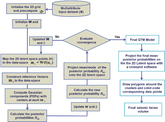
Generative
Tomographic Mapping
A non-linear dimension reduction technique, an extension on SOM
GTM estimates the probability that a data vector is represented by a grid point or node in the lower dimensional latent space
Example:
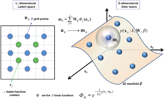
2D (L=2-dimensional) latent space with 9 nodes ordered on a regular grid and 4 basis function centres on the left. Each node in the latent space is defined by a linear combination of a set of J nonlinear basis functions φj (Gaussian), also spaced regularly. The nodes are projected on a 2D (L=2-dimensional) non-Euclidean manifold S in the (D-dimensional) data space, on the right. Each grid point uk is mapped to a corresponding reference vector m
k on the manifold S in data space. Data vectors xn are scattered in data space. To fit the data vectors to manifold S, isotropic pdf’s centred at mk are assumed. The total pdf at point xn in the data
space is the combination of all pdfs of the mk’s at the data point. On the other hand, each mk has a finite probability of representing xn.
Using expectation maximization (EM) clustering, each mk moves toward the nearest data vector xn
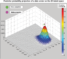
With this prior probability value at each mk, using Bayes rule, posterior probabilities are calculated for each m
k., showing the probability that it represents the data point. These probabilities are then assigned to the corresponding uk in the latent space. In the right plot, the posterior probability distribution for 1 data vector
x
n in the 2D latent space is shown. The mean and the mode are shown. The mean of data vectors form clusters in the latent space.
Given labelled data in each cluster, GTM can also be used for supervised classification
Procedure:
Geophysical
curiosity 41
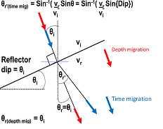
A nice illustration of the difference between time migration and depth migration is shown in the figure on the left. Time migration assumes the reflector to be locally flat, as its basic assumption is that the velocity model consists of horizontal layers. Hence, a ray with normal incidence on the dipping layer will be refracted according to the horizontal interface, whereas in depth migration the normal incidence ray will not be refracted (will continue in the same direction).
Geophysical
curiosity 40
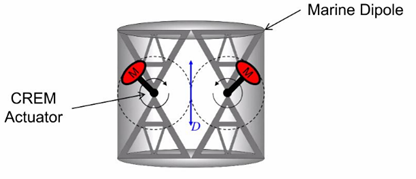
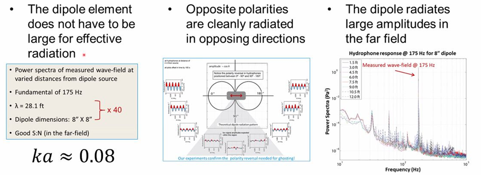
It is well known that low frequencies are
essential for Full Waveform Inversion (FWI). During the 3rd GSH/SEG Symposium,
I came across a remarkable piece of research related to the generation of low
frequencies in a marine environment. The source is a dipole source generated by
two counter-rotating masses, radiating low frequency acoustic waves. The Dipole
Marine Source does not generate changing volumes. In the far-field the ghost
from the sea surface is in phase with the primary signal and thus enhances the
signal strength. In total it adds two or more octaves at the low frequency
side. The concept was tested and proven to be working, but unfortunately it was
never put into active application.
Ref.: Frontiers in low frequency seismic
acquisition, Mark Meier, 3rd GSH/SEG Web Symposium, 2021
It is well known that low frequencies are
essential for Full Waveform Inversion (FWI). During the 3rd GSH/SEG Symposium,
I came across a remarkable piece of research related to the generation of low
frequencies in a marine environment. The source is a dipole source generated by
two counter-rotating masses, radiating low frequency acoustic waves. The Dipole
Marine Source does not generate changing volumes. In the far-field the ghost
from the sea surface is in phase with the primary signal and thus enhances the
signal strength. In total it adds two or more octaves at the low frequency
side. The concept was tested and proven to be working, but unfortunately it was
never put into active application.Geophysical curiosity 39
Robust Estimation of Primaries by Sparse Inversion (EPSI) avoids these difficulties by solving directly for the multiple-free wavefield. It seeks the sparsest surface-free Green’s function in a way that resembles a basis pursuit optimization. In addition, it can find solutions in arbitrary transform domains, preferably ones with a sparser representation of the data (for example, curvelet transform in the spatial directions and wavelet transform in the time direction). It can also handle simultaneous-source data.
As the Green’s function is expected to be impulsive, the method uses the sparsity of the solution wavefield as the regularization parameter. By reformulating EPSI under an optimization framework, the “Pareto analysis” of the Basis Pursuit Denoising optimization can be used.
Wikipedia:
Basis Pursuit Denoising (BPDN) refers to mathematical optimization. Exact solutions to basis pursuit denoising are often the best computationally tractable approximation of an underdetermined system of equations. Basis pursuit denoising has potential applications in statistics (Lasso method of regularization), image compression and compressed sensing.
Lasso (Least Absolute Shrinkage and Selection Operator) in statistics and Machine learning is a regression analysis method that performs both variable selection and regularization to enhance the prediction accuracy and interpretability of the resulting statistical model.
Lasso was originally formulated for linear regression models.
Pareto analysis is a formal technique useful where many possible courses of action are competing for attention. In essence, the problem-solver estimates the benefit delivered by each action, then selects a number of the most effective actions that deliver a total benefit reasonably close to the maximal possible one.
Hence, it helps to identify the most important causes that need to be addressed to resolve the problem. Once the predominant causes are identified, then tools like the “Ishikawa diagram” or “Fish-bone Analysis” can be used to identify the root causes of the problem. While it is common to refer to pareto as "80/20" rule, under the assumption that, in all situations, 20% of causes determine 80% of problems, this ratio is merely a convenient rule of thumb and is not nor should it be considered an immutable law of nature. The application of the Pareto analysis in risk management allows management to focus on those risks that have the most impact on the project.
Ref: Lin & Herrmann, Robust estimation of primaries by sparse inversion via L1 minimization. Geophysics, 2013, V78, N3, R133–R150.
Geophysical curiosity 38
The core idea of GAN is based on the "indirect" training through the discriminator, which itself is also being updated dynamically. This basically means that the generator is not trained to minimize the distance to a specific image, but rather to fool the discriminator. This enables the “model” (ML terminology) to learn in an unsupervised manner.
The generative network generates candidates while the discriminative network evaluates them. The contest operates in terms of data distributions. Typically, the generative network learns to map from a latent space (containing the distributions of the features of the real data) to a data display of interest, while the discriminative network distinguishes candidates produced by the generator from the true data. The generative network's training objective is to increase the error rate of the discriminative network (i.e., "fool" the discriminator network by producing novel candidates that the discriminator thinks are not synthesized, but are part of the true data set).
A known dataset serves as the initial training data for the discriminator. Training it involves presenting it with samples from the training dataset, until it achieves acceptable accuracy. The generator trains based on whether it succeeds in fooling the discriminator. Typically, the generator is seeded with randomized input that is sampled from a predefined latent space (e.g., a multivariate distribution). Thereafter, candidates synthesized by the generator are evaluated by the discriminator. Independent backpropagation procedures are applied to both networks so that the generator produces better samples, while the discriminator becomes more skilled at flagging synthetic (fake) samples.
An example of a GAN network with a Generator and a Discriminator
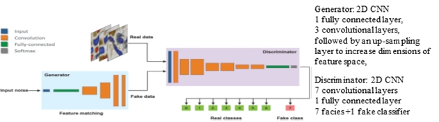
“Real” and “Fake” data, with fake data generated by the Generator network can be presented to the Discriminator, which must decide what the real class (0-6) of the sample is or whether it is fake (7). The Generator samples randomly from a latent space which contains the distributions related to the real samples, construct a seismic display, and presents it to the Discriminator. If the Discriminator decides it is fake, it will feed that back to the Generator. In the iterations both networks try to improve their performance: The Generator to construct seismic that fools the Discriminator, and the Discriminator to discriminate real from fake. After many epochs, a set quality criterium will be reached defining the final Generator and Discriminator. Note over- and under-fitting should be avoided.
Stated otherwise:
1.The generator tries to create samples that come from a targeted yet unknown probability distribution and the discriminator to distinguish those samples produced by the generator from the real samples.
2. The generator G(z,\( \Theta \) g) extracts a random choice from the latent space (of random values) and maps it into the desired data space x.
3. The discriminator D(x,\( \Theta \)d) outputs the probability that the data x comes from a real facies.
4. \( \Theta \) g and \( \Theta \)d are the model parameters defining each neural network, which need to be learned by backpropagation.
5. When a real sample from the training set is fed regardless of being labelled or unlabelled, into the discriminator, it will be assigned a high probability of real facies classes and a low probability of fake classes, whereas it is the opposite for samples generated by the generator.
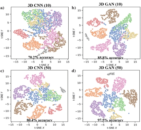
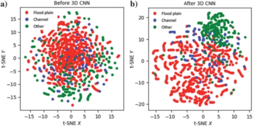
Below is shown an example comparing a stand-alone CNN with a GAN. It shows the seismic facies distribution before and after applying 3D CNN and 3D GAN with 10 and 50 labelled samples per class (10 makes up a very limited training data set). The displays lead to the following conclusions: 1) CNN as well as GAN result in a much better separation between the classes/facies, 2) the larger the training data set the better the performance (% accuracy) and 3) GAN performs better than 3D CNN in case of a limited learning set.
What happens after training & validation? If the aim is the increase the Learning dataset, then the Generator can be used to create additional samples. If the purpose is to classify the rest of the seismic cube, then we discard the Generator and use the trained Discriminator.
Ref: Liu et al., Geophysics 2020, V85, N4
Geophysical curiosity 37
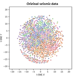
Finally, I found a publication (Liu et al., Geophysics 2020, V85, N4) which showed me several nice examples, using a display called t-SNE (See below for a description). The display has the same characteristics a Self-Organised-Map (SOM) in that instances or samples that are closely located in the multidimensional attribute space are mapped close together in a lower dimensional (2D or 3D) space.
Below is an example showing the facies distribution in 2D for seismic before and after CNN. The CNN “attributes” show a better separation between the different facies.
https://en.wikipedia.org/wiki/T-distributed_stochastic_neighbor_embedding
Geophysical curiosity 36
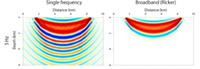 Let us look at the way the energy travels from
shot to receiver. On the left we see the sensitivity kernel for a single frequency. By interference we have the fundamental and the higher order “Fresnel zones” along which the energy travels, by constructive interference. On the right we see
that for a broadband signal the higher order Fresnel zones have disappeared by destructive interference. But we do not have a pencil sharp ray-path, rather a fat ray or Gaussian beam.
Let us look at the way the energy travels from
shot to receiver. On the left we see the sensitivity kernel for a single frequency. By interference we have the fundamental and the higher order “Fresnel zones” along which the energy travels, by constructive interference. On the right we see
that for a broadband signal the higher order Fresnel zones have disappeared by destructive interference. But we do not have a pencil sharp ray-path, rather a fat ray or Gaussian beam.
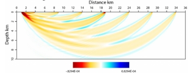 Another example shows turning waves going from
shot to different receiver locations, shown as “fat rays”. Again, the ray area/volume shows which part of the subsurface influences the wave propagation and thus can be updated using the difference between modelled and observed wave phenomenon,
using inversion minimising a loss function.
Another example shows turning waves going from
shot to different receiver locations, shown as “fat rays”. Again, the ray area/volume shows which part of the subsurface influences the wave propagation and thus can be updated using the difference between modelled and observed wave phenomenon,
using inversion minimising a loss function.
Let us look at another geophysical phenomenon: Full Waveform Inversion or FWI for short, where we model the complete wavefield and compare the modelled wavefield with the observed one to update the model parameters. What does the sensitivity kernel
look like?
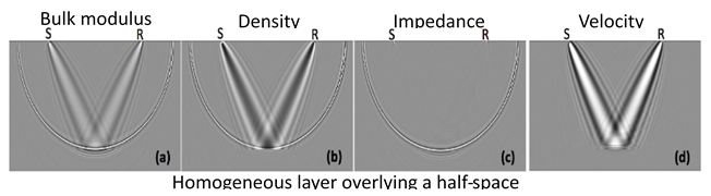
For a homogeneous overburden above a reflector at 4 km depth the sensitivity kernel is shown below.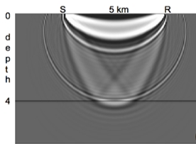 We observe basically 3 parts. An ellipse, a banana shape and so-called rabbit ears. The ellipse is related to scattering from the interface at 4 km depth,
the banana shape deals with turning waves and the rabbit ears relate to to the reflection from the interface. The rabbit ears are usually an order of magnitude smaller in amplitude as they are scaled by the reflection coefficient. As seen
in figure d above, they deal with the low spatial wavenumbers of the velocity and density above the reflector, or in other words with the background model.
We observe basically 3 parts. An ellipse, a banana shape and so-called rabbit ears. The ellipse is related to scattering from the interface at 4 km depth,
the banana shape deals with turning waves and the rabbit ears relate to to the reflection from the interface. The rabbit ears are usually an order of magnitude smaller in amplitude as they are scaled by the reflection coefficient. As seen
in figure d above, they deal with the low spatial wavenumbers of the velocity and density above the reflector, or in other words with the background model.
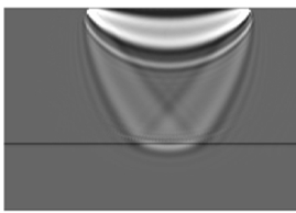 We clearly have suppressed the part related
to the specular (single point) reflection/scattering, although not completely as can be seen just above the reflector.
We clearly have suppressed the part related
to the specular (single point) reflection/scattering, although not completely as can be seen just above the reflector.
This suppression is obtained by applying so-called dynamic (time-varying) weights to the velocity sensitivity kernel.
So, by suppressing the high wavenumber parts not related to the background velocity model we will enhance the sensitivity to the low wavenumber components in the response. Using that response, the background velocity can be updated by minimizing
the difference between the observed and the model background velocity.
This is also called “separation of scales”.
Ref: Martin et al., FB, March 2021
Martin et al., EAGE 2017, Th B1 09
Ramos-Martinez et al., EAGE 2016, Th SRS2 03
Geophysical curiosity 35
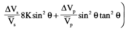

R(\( \Theta \)) can be expressed as ½\( \Delta \)EI/EI=½\( \Delta \)ln(EI), this results in:
EI(\( \Theta \))=Vp(1+tan²\( \Theta \))Vs(-8Ksin²\( \Theta \))\( \rho \)(1-4Ksin²\( \Theta \))
Neglecting the third term in the linear approximation results in:
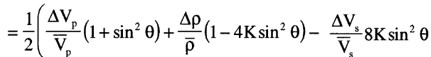
EI(\( \Theta \))=Vp(1+sin²\( \Theta \))Vs(-8Ksin²\( \Theta \))\( \rho \)(1-4Ksin²\( \Theta \))
So, replacing tan2\( \Theta \) by sin2\( \Theta \) in the EI expression is equivalent to ignoring the third term in the linear approximation.
Note that for K=0.25, EI(90°)=(VP/VS)2 in the last expression.
Ref: Conolly, The Leading Edge 1999, V18, N4, P438-452.
Another simplification, based on neglecting the third term is given in
Veeken & Silva, First Break 2004, V22, N5, P47-70.
Geophysical curiosity 34
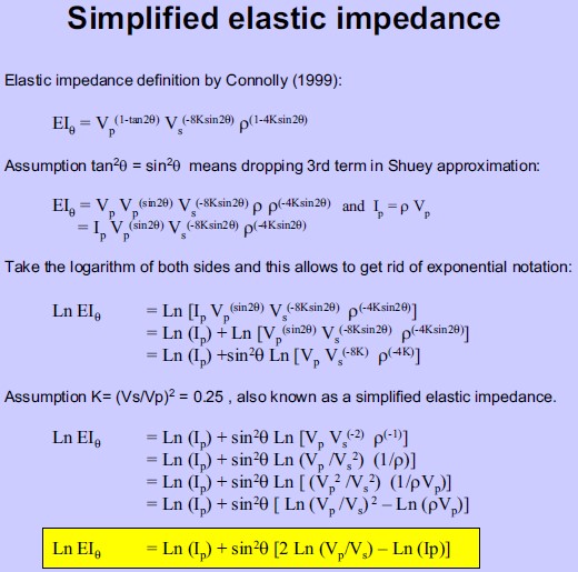
Given a plane interface between two anisotropic TVI media. That means in each medium we have different vertical and horizontal velocities: V1v, V1h, V2v and V2h .
Question: Which velocities are used
to describe Snell’s law?
Answer: Ref: James, First Break 2020, V38, N12 
Based on the above figure, the following relationships can be derived:
sin\( \alpha \)2=AD/AB and sin\( \alpha \)1=BC/AB ,
or
AD=ABsin\( \alpha \)2 and BC=ABsin\( \alpha \)1 ,
hence
tAD=AD/V2h=ABsin\( \alpha \)2/V2h
and tBC=BC/V1h=ABsin\( \alpha \)1/V1h
as tAD=tBC it follows that ABsin\( \alpha \)2/V2h =ABsin\( \alpha \)1/V1h or sin\( \alpha \)2/V2h =sin\( \alpha \)1/V1h .
This is Snell’s law, but involves the horizontal velocities.
A generalisation showing that Snell’s law is valid for any anisotropic medium.
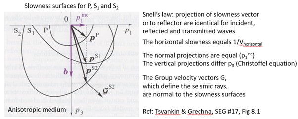
Note that for a horizontal interface the projections
equal the horizontal velocities, otherwise they are the velocities parallel to the interface at the reflection/transmission point.
Geophysical curiosity 33
Performing the wavefield separation above the sea floor results in an
- Up-going wavefield containing the primary reflections, refractions and all multiples other than receiver-side ghosts and a
- Down-going wave field containing the direct arrivals plus the receiver-side ghosts of each upgoing arrival.
Another use of separating the wavefields is to deconvolve the upgoing wavefield by the down-going wave field. This has the following advantages:
- Fully data-driven attenuation of free-surface multiples without acquiring adaptive subtraction
- Mitigating the effects of time- and space-varying water column velocity changes (4D)
-
Deconvolves the 3D source signature in a directionally consistent manner.
Geophysical curiosity 32
Physics Informed Neural Networks (PINN)
A disadvantage of the “traditional” Neural Networks is that the resulting model might not satisfy the physics of the problem considered. Luckily, there are 2 ways of overcoming this issue,
using as an example the eikonal equation.
One way is to use synthetic data that has been generated using physics. For example, if the travel-time data from a source to multiple receiver points (x, y, z) are calculated using the eikonal equation, then the relationship between a velocity model and the travel-times satisfies the physics of wave propagation. If that (training) data is used to build a machine learning model, then that model will satisfy the underlying physics. The Neural network, we will use, consists of 3 input nodes (x, y, z) and one output node (Travel time) and will be trained using many receiver locations. This model can then be used to calculate the travel times for other locations in the same model or even for calculating travel times in other velocity-depth models (Transfer Learning).
The other way is to include the eikonal equation in the loss function. That means that the loss function now consists of an eikonal expression, a data difference between observed and estimated travel time and a regularization term. The resulting ML model will (to a very large degree) satisfy the wave propagation physics. Note that in this case the data even does not need to be labelled, that means the data does not need to contain the true travel times.
An interesting application is to build a ML model for determining the source location for observed arrival times. Using distributed source points in a velocity-depth model the algorithm can be trained to find the source points from the observed times. Applying this algorithm to a new micro-seismic event, the location of this event can then be predicted (in no time, as the application of a ML model needs very little compute time).
Geophysical curiosity 31
Vector Magnetic Data
In Airborne Gravity we use the three components of the gravity field (Full Tensor Gravity) measurements extensively. In Airborne Magnetics the low precision of the aircraft attitude hindered the use
of multi-component magnetic data. With a novel airborne vector magnetic system (Xie et al, TLE 2020, V39, N8) the three components can be recorded with sufficient high Signal-to-Noise ratio to allow accurate calculation of geomagnetic inclination
and declination.
In test flights the new system has a noise level of 2.32 nT. The error of repeat flights was 4.86, 6.08 and 2.80 nT for the northward, eastward and vertical components.
A significant step forward.
Geophysical curiosity 30
Bayes Rule
A joint distribution of two random variables A & B is defined as P(A∩B). If the two random variables were independent than P(A∩B)=P(A)P(B). However, when the variables are not independent, the joint distribution
needs to be generalized to incorporate the precedent that we either observe A with knowledge of B or vice versa. Bayes’s theorem guarantees that the joint distribution is symmetric in relation to both situations, that is:
P(A)P(B|A)=
P(A∩B)= P(B)P(A|B)
Bayes’s rule is seldom introduced in this way. Ref Jones, FB219, Issue 9
Geophysical curiosity 29
Rock Physics
The wave equation is derived by combining constitutive and dynamical equations. The constitutive equation defines the stress-strain relationship and the dynamical equation shows the relation between force and acceleration.
The most-simple constitutive equation is Hooke’s law (\( \sigma \)=C.\( \epsilon \), with C the stiffness matrix, or \( \epsilon \)=S.\( \sigma \), with S the compliance matrix, S=C-1). All the medium properties can be defined in
the stiffness matrix, thus also all kinds of anisotropy: Polar (5), Horizontal (5), Orthorhombic (9), Monoclinic(12) and Triclinic (21) anisotropy, where the numbers indicate the number of independent matrix components. 5 for horizontal
layering, 9 for horizontal layering with vertical fractures, 12 for horizontal layering and slanting fractures and 21 for the most general case. So, the stiffness matrix makes the wave equation complicated. In addition, it is whether we consider
the acoustic, visco-elastic or poro-elastic case which further complicates the wave-equation.
The poro-elastic model is the least known. It is maybe not so relevant for seismic wave propagation, as the frequencies are low. But in the
kHz range it can not be ignored. The difference is because at low frequencies the pore fluids moved together with the rock, whereas at high frequencies the pore fluid tend to stay stationary, that means move relatively in the opposite direction.
Now here comes the important part. In a poro-elastic medium there exists a fast P-wave (fluid moves with the rock) and a slow P-wave (fluid moves in opposite direction). So, in principle, if we could measure the slow wave, we might be able
to conclude something about the permeability, namely the lower the permeability the less the pore fluid can flow in the opposite direction. Hence, maybe one day…
Geophysical curiosity 28
Gramian constraints
Although I only became aware recently, Gramian constraints have been used for many years now. What are Gramian constraints and where are they applied?
Gramian constraints are used in inversion as
one of the terms in the loss function. Inversion tries to find the model parameters that minimize a loss function. In a loss function several terms can be present: difference between the observed and the modelled data, difference between starting
and latest updated model, smoothness of model and Gramian constraints.
Gramian constraints use the determinant of a matrix in which the diagonal elements are autocorrelations of the model parameters and the off-diagonal elements the
cross correlations between the parameters. These parameters are normalised (weighted), which is especially important if they have different magnitudes as in the case of joint inversion of different data sets (seismic, gravity, magnetic, EM)
In
the minimization of the loss function, parameter values are searched for which among others aims for a minimum of the determinant, which means tries to maximize the off-diagonal elements. This means it tries to increase the cross-correlations
between the parameters. It will only be able to do so within the restrictions: other terms in the loss function shouldn’t start increasing more than the decrease in the Gramian term and it will only increase the off-diagonal terms if the data
indicate cross-correlations exist. Hence, the use of the expression “It enhances the cross-correlation (if present)”.
Note that the Gramian can be based on the parameters, but also on attributes derived from the parameters (e.g. log(parameter)).
It is useful to linearize the relationship as cross-correlations relate to linear relations only.
When also spatial derivatives of model parameters are used, we can incorporate coupling of structures of different properties (cross-gradient
minimization).
Geophysical curiosity 27
Jan. 31th 2020
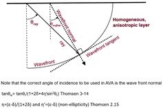
Ray or wavefront angle for AVA?
The question is, should we be using the ray or the wavefront angle of incidence on the interface when we apply the Zoeppritz equations. In case of a homogeneous subsurface, rays (high frequency
approximation) are perpendicular to the spherical wave fronts. This is even so for inhomogeneous media, although the wave fronts will no longer be spherical.
For anisotropic media we distinguish a difference between a ray and wave front normal direction, and also between the wavefront normal velocity (phase velocity) and energy propagation velocity (ray velocity).
As the wavefront can be considered
the result of constructive interference of plane waves, it follows that the angle of incidence of the wavefront normal on the interface should be used in the Zoeppritz calculations.
However, when we plot AVA, we usually plot the reflection
amplitude as function of the angle of departure from the surface, hence the ray angle again. See the display below from the 2002 Disk course by Leon Thomsen.
Geophysical curiosity 26
Reading the article “CSEM acquisition methods in a multi-physics context” in the First Break of 2019, Volume 37, Issue 11, the following question, which has been bothering me for some time, came up: An EM field has coupled electrical and magnetic
components. The information in both is the same. So, we can measure either E or H and will receive the same information on the subsurface. If so, why not use H as the (x,y,z) receiver instruments are much smaller and operationally easier to
use. Is the signal-to-noise ration the issue?
I was pleased to receive the following answer from Lucy MacGregor: You’re absolutely right. The signal contains both E and H fields and they contain much the same information. There have
been various modelling studies that have demonstrated that electric fields are generally used in preference to magnetic fields precisely because of signal to noise ratio. Magnetic fields are much more susceptible to motional noise. Overcoming
this was the reason Steve Constable started using huge concrete weights. He needed to keep the instruments still to record magnetic fields for MT. For this reason, it would be hard to put magnetic field sensors in a cable, all you would see
is cable motion. Now, of course E fields are also susceptible to cable motion, but you can get over this by using a relatively long dipole to average it out (which is what PGS did and that worked well).
In addition, I like to mention
that in a later article in the same issue, vertical pyramidal structures were used to stabilise the vertical long E dipoles placed on the seafloor.
Geophysical curiosity 25
Jan. 10th 2020
Non-seismic geophysics gets on average little attention in the industry. Although seismic is the main method in many applications in the energy industry, non-seismic methods play a more dominant role in geothermal energy, pollution mitigation and certainly with respect to mineral exploration.
In the forthcoming energy transition, rare-earth elements are essential. Having them available will be an important (political) item in the future. Therefore, non-seismic geophysical methods will become more important. An interesting example can be found on the following website:
http://www.sci-news.com/geology/mountain-pass-rare-earth-element-bearing-deposit-07987.html
Geophysical curiosity 24
Spatial sampling
An interesting new development from TesserACT.
Nyquist’s theorem has been the guiding force behind a relentless striving to achieve ever more regular sampling geometries. Over the last few years, “compressive
sensing” has challenged this orthodoxy. In lay man’s terms, compressive sensing offers the promise of stretching Nyquist a little in order to achieve better data quality (or lower cost) by removing the artefacts created by regular grids:
Conventional
acquisition:
shots & receivers Randomized acquisition: shots &
randomized receivers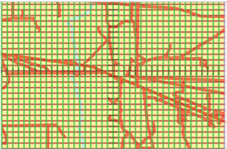
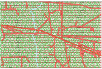
Conventional acquisition: shots & receivers Randomized
acquisition: randomized shots & receivers
Although it has been known for a long time that the Nyquist restriction could be relaxed by randomization, it is only due to more accurate & efficient positioning
that the application became operationally feasible.
Geophysical curiosity 23
New Terminology
To work with the hottest topic of today, that is Machine learning, one needs to familiarize oneself with new terms. Often it is a matter of semantics, using a different name for a well-known item. This unfortunately
acts as a barrier. Examples are feature for attribute, instance for case, etc. It starts already with the name Machine Learning. Years ago, I learned about Pattern Recognition, then later it was called Artificial Intelligence. Now it is Machine
Learning or Deep Learning. Only a matter of getting used to.
Geophysical curiosity 22
April 24th 2019
Steerable total variation regularization
In signal processing, total variation regularization (TV), is based on the principle that signals with excessive and possibly spurious detail have high total variation, that is, the
integral of the absolute gradient of the signal is high. According to this principle, reducing the total variation of the signal, subject to staying close to the original signal, removes unwanted detail whilst preserving important details
such as sharp contrasts.
This noise removal technique has advantages over simple techniques such as linear smoothing or median filtering (although also known to be edge preserving), which reduce noise but at the same time smooth away edges to a greater or lesser degree. By contrast, total variation regularization is remarkably effective at simultaneously preserving edges whilst smoothing away noise in “flat” regions, even at low signal-to-noise ratios.
Total Variation is used in FWI to regularize the output of the non-linear, ill-posed inversion.
A new development in TV is steerable total variation regularization. It allows steering the regularization of the FWI solution towards weak or strong
smoothing based on prior geological information.
Hold-on, doesn’t that lead to a very pre-conceived result. That could indeed be the case when not done carefully.
However, there is a way in which it can be done by including that prior information in the regularization parameter rather than in the misfit term as done usually. A spatially variant regularization parameter based on prior information where sharp contrasts are expected can be used. It will first reconstruct the high contrasts (salt bodies) followed by filling in the milder contrasts (sediments) at later stages.
Ref: Qui et al, SEG2016, P1174-1177
Geophysical curiosity 21
April 24th 2019
Wasserstein distance
A most curious metric
In Full-Waveform Inversion the subsurface model is updated by minimizing the difference between synthetic/modelled and observed data. This is usually done by a sample-by-sample
comparison (trace-by-trace or globally) using the L2-norm. The advantage of the L2-norm is that it is an easily understood and fast comparison, the disadvantage is that the model update is prone to errors due to poorly updating the low wavenumber
trends, also mentioned as cycle skipping (more than half-wavelength shifts). Several ways of overcoming this issue are available. The most common one is to use a multi-stage approach, in which we start with the lowest available frequency (longest
wavelength=largest time difference for cycle skipping) and then using increasing frequencies (Hz) in subsequent stages (2-4, 2-6, 2-8, 2-10, etc).
Now recently, at least for geophysics, a new difference measure has been used with great
success, the quadratic Wasserstein metric W
2. This metric appears to me as curious. It namely computes the cost of rearranging one distribution (pile of sand) into another (different pile of sand) with a quadratic cost function (cost depends for each grain on the distance
it needs to be moved/transported). This explains the term “optimal transport” which is often mentioned.
The advantage of using the W2 metric is that the cost function is much more convex (a wider basin of attraction), mitigating
cycle skipping and hence less sensitive to errors in the starting model.
However, some extra data pre-processing is needed to apply this method. The synthetic/modelled and observed data need to be represented as distributions, which
means non-negative and sum-up to unity. This can easily be achieved.
Another interesting approach is not to use the samples themselves, but first map the data to another more “suitable” domain, for example the Radon domain.
And
then there is another “unexpected” improvement by not using the samples themselves, but by using the matching filter between observed and modelled data. If the two are equal, the matching filter would be a delta function. Hence, the model
update is done by minimizing the Wasserstein distance between the matching filter and a delta function (for stability a delta function with a standard deviation of 0.001 is used). And apparently, this cost function allows updating the subsurface
model.
Great, isn’t it.
Ref: Yang et al., Geophysics, 2018, V83, N1, P.R43-62
Geophysical curiosity 20
Matching Pursuit
How to explain matching pursuit?
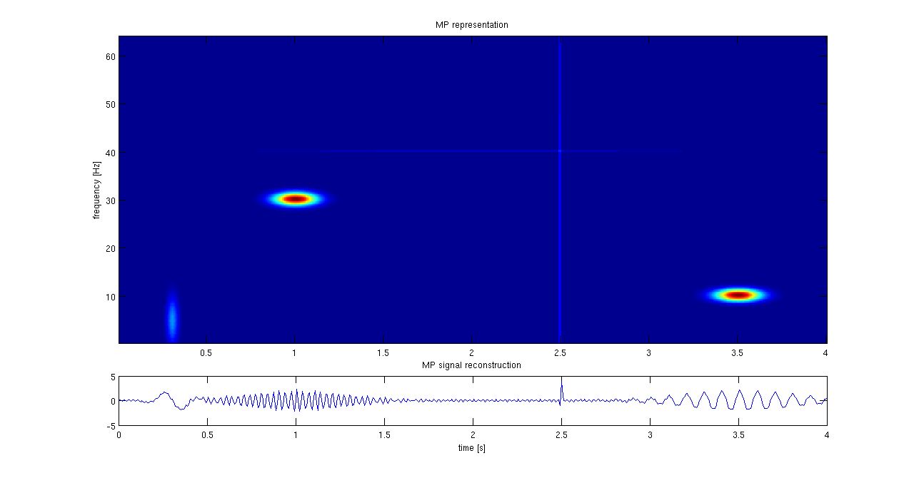
I will use the
above plot from Wikipedia to explain matching pursuit. Given a time signal, we like to decompose it into a minimum number of components. The number of possible components, contained in a dictionary, is large, not to say unlimited. So, I start
by matching the signal first with the most important, best matching component, then I take the next one and I keep on doing this, I pursue to get a better match, till I am satisfied with the match, which means the signal has been sufficiently
approximated using “only” N components.
In the example above, the axes are time vs frequency, the components are cosine functions in the frequency range 0-60 Hz and the results show that time signal can be well represented by the centres
of the ellipses.
Geophysical curiosity 19
April 2th 2019
Inversion of seismic data
The simplest definition of seismic data inversion I came across is:
“Going from interface to Formation information”
Geophysical curiosity 18
Do shear waves exist in an acoustic medium?
This is a curious question as it is well known that shear waves do not exist in an acoustic medium, because that is the “definition” of an acoustic medium? In an acoustic medium \(
\mu \) equals 0, hence V2S= \( \mu/ \rho=0 \), which means shear waves cannot propagate and hence cannot exist.
But another definition of an “acoustic” medium is also used (Alkhalifah, Geophysics, V63, N2, P623-631),
namely defining it by V
S0=0, that is the vertical shear wave velocity equals 0. This definition of acoustic is used to simplify the equations for P-wave propagation. However, it defines the medium to be truly acoustic for an isotropic medium only. In
case of VTI anisotropy the story is different. Namely, in that case a shear wave exists as demonstrated by the (phase velocity) expression below: Grechka et al, Geophysics Vol 69, No.2, P576-582.
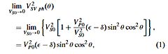
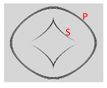
Fig.1: Wavefronts at 0.5 s generated by a pressure source
in VTI medium with VP0=2 km/s, VS0=0 and \( \epsilon \) =0.4, \( \delta
\) =0.0
From the formula we see that except for the vertical (\( \Theta \)=0°, 180°) and horizontal (+/-90°) directions a SV wave exists in case \( \epsilon \neq \delta \) (the VTI anisotropy is not “elliptical”). Wavefront modelling (Fig.1) indeed
shows that a curious shear wavefront is generated in accordance with expression (1).
Hence, defining the medium to be “acoustic” by putting the vertical shear wave velocity (VS0) to zero simplifies the P-wave equations, but
do not make the medium truly acoustic. For anisotropic media, shear waves, are still excited in the medium. For modern high-resolution seismic modelling, the “noise” generated is not negligible.
Thus, putting VS0=0 doesn’t
make the medium truly acoustic in case of anisotropy.
P.S. To be fair to Alkhalifah he called it an acoustic approximation.
Geophysical curiosity 17
Feb. 20th 2019
Cloud computing in Geophysics
Cloud computing is hardly used in geophysical processing. Whether that is due to security issues or the amount of data involved is not clear to me. Interestingly enough a recent publication by Savoretti et al, from Equinor in the first Break, V36, N10 gives some insight in the approach.
It is well known that cloud computing provides access to a scalable platform, servers, databases and storage options over the internet. The provider maintains and owns the network-connected hardware for these services.
It offers increased flexibility in access to compute power and data sets are easily transferred to the cloud during project work and removed afterwards. In cluster terms an allocated compute node participates in running workloads via a queue system, which keeps track of what can be done on which node most efficiently.
What I didn’t know is how it is commercially arranged. It appears that nodes can either be ordered permanently or from a “spot market” for lower prices. However, spot market nodes can be taken away suddenly in case there is a higher bidder. The work done so far on that node will then be lost.
To minimize the effect, the workflow has been adjusted to better tolerate loss of nodes in spot-market environment. Since then better use can be made of the cheaper spot-market nodes by automatic recovery and more fully automated mode ordering.
Geophysical curiosity 16
Dec. 24th 2018
Machine learning
Machine Learning, also called Artificial Intelligence or Algorithms, is today’s hot topic. It is also associated with “Big Data”, indicating that its use can mainly be found in case an overwhelming amount of
data need to be explored.
Is Machine Learning also useful in geophysics? Before answering this question, I like to pose another question: Will Machine learning replace the Physics in Geophysics? By that I mean do we still need formulae and equations to explore
for hydrocarbons, salt/fresh water, polluted/unpolluted subsurface, etc? To answer this question let’s look at “traditional” versus “new” geophysics.
In the traditional geophysics we try to interpret observations / data by applying
two main methods: forward modelling and inversion. In forward modelling we assume a (best guess) model of the subsurface and use equations, like the visco-acoustic wave equation for seismic, to derive related observations (synthetic data).
By comparing these synthetic data with the real observations, we derive an update of the assumed model using inversion. The success depends heavily on the accuracy (adequacy) of the forward modelling and the ability of solving the ill-posed
inversion. So, it is essential to fully understand the physics of the problem.
In Machine Learning it is different. An understanding of the physics is useful, but not essential. It is now a matter of having a sufficiently large learning
/ labelled data set which (hopefully) contains a statistical relationship between the observations and the related subsurface. This relationship, which is nothing else than a “correlation”, will be derived by a clever algorithm that contains
parameters, which are determined by tuning the algorithm using the learning (labelled) data set. This tuning will determine the parameter values resulting in a predictive capability of the algorithm with an appropriate accuracy. Among the
numerous kinds of algorithms, the most popular ones are called Neural Nets.
Neural Nets consist of an input layer, hidden layers and an output layer, each containing nodes.
An input node is fed with a seismic sample or an 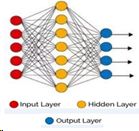 attribute /feature from a point in the 3D data set. A node in a hidden layer would receive weighted inputs from all input nodes and depending on the sum provide input to the nodes in the output layer. Each node in
the output layer represents a class, say lithology or fluid saturation of a reservoir interval. The sum of each output node would indicate whether the input belongs to its class. In the learning phase the weights will be determined. Once determined,
the network would be able to predict the class /character of new input data (undrilled locations). It can also be used in an unsupervised way to determine clusters of data, which then still need to be interpreted. In general, more hidden layers
are needed to be able to handle more difficult problems.
attribute /feature from a point in the 3D data set. A node in a hidden layer would receive weighted inputs from all input nodes and depending on the sum provide input to the nodes in the output layer. Each node in
the output layer represents a class, say lithology or fluid saturation of a reservoir interval. The sum of each output node would indicate whether the input belongs to its class. In the learning phase the weights will be determined. Once determined,
the network would be able to predict the class /character of new input data (undrilled locations). It can also be used in an unsupervised way to determine clusters of data, which then still need to be interpreted. In general, more hidden layers
are needed to be able to handle more difficult problems.
Now, if you like the physics of geophysics, that is formulae and equations give you a warm feeling as they are an unambiguous, short and clear language describing physical processes,
then you will have a tendency to give preference to traditional geophysics, but if you need practical results to earn an income (say predictions of fluid saturations in carbonates), then you will have to rely on the benefits of applying machine
learning in addition to an understanding of the underlying physics.
So, the answer to the question: “Which one will be the winner?” will be in my opinion: Neither of the two, it will be a combination of both.
Geophysical curiosity 15
Quaternion
Up to now I didn’t know of the existence of quaternions and that they can also be used in geophysics. What is a quaternion?
A complex number is defined as a+ib, a quaternion as q=a+bi+cj+dk, hence it is a hypercomplex number.
It allows
a Fourier domain representation of multi-component seismic data. For example, so-called “Projection Onto Convex Sets” (POCS) reconstructs all three seismic components at once.
Applications are in image disparity methods (edge detection),
interpolation, time-lapse analysis, separation of up- and down-going waves (VSP) and calculation of attributes.
However, so far I have encountered very few “real” applications.
Geophysical curiosity 14
Migration or Wavefield reconstruction versus Imaging
It is important to make a distinction between wavefield reconstruction and imaging.
Migration is a two-step process: 1) wavefield reconstruction and
2) imaging.
Wavefield reconstruction is the determination of the wavefield over a volume of interest. Imaging involves the making of a picture of the geometrical distribution of the reflecting surfaces within the medium.
This is best illustrated
by the fact that we perform a downward continuation, forward in time, of the wavefield generated by a source and a downward continuation, but now backward in time, of the recorded wavefield, followed by the application of an imaging condition
to obtain the reflection point in space and its reflection strength.
Again, we have various methods for wavefield continuation, the more sophisticated the more accurate (acoustic, elastic, visco-elastic) and various so-called imaging
conditions (cross-correlation, deconvolution, least-squares deconvolution).
Geophysical curiosity 13
Question: Is seismic a hologram?
Hologram
An optical hologram is not an image; it is a recording of a wavefield. Remember how a hologram is made: A single frequency laser light is split into two parts.
One part is mirrored directly onto the recording plate; the second one is reflected / diffracted by the object. What is recorded on the plate is the interference pattern between the two.
When we beam the laser onto the “developed” plate
and look through we see the object in 3D. Looking from different directions we see the object from these different directions. Even more fascinating is that when we break off a part of the plate, we can still see the total object from all
directions, although the smaller the remaining piece the poorer the quality of the image.
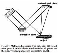
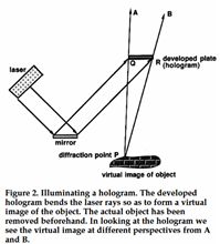
Seismogram
Remember that in seismic
we can consider the subsurface to consist of a collection of diffraction or scattering points. This would imply that a single shot recorded by a single geophone would record diffraction energy from any point of the subsurface. Hence, the single
record contains information about the entire subsurface and it would be possible, in principle to reconstruct/image the complete subsurface. This is like the concept that a single point on a hologram is enough to observe the object in 3D.
But again, we would prefer a larger piece of the plate, i.e. more observations, to obtain a better-quality image.
Lesson learned
If we would apply holographic seismic imaging, we could do with a much sparser and
therefore cheaper survey.
Ref.:
“Extended resolution: Neidell is right”, E.A. Robinson, TLE 2018V37, N1
‘holistic migration”, E.A. Robinson, TLE 1998, V17, N3
Added statements by Öz Yilmaz
“Spatial under sampling
can be compensated by temporal oversampling”
“Temporal oversampling enables the extension of the spectral bandwidth beyond the Nyquist frequency”
Geophysical curiosity 12
What is the difference between updating a velocity model in the data or in the image domain? Are we using the same data?
Updating of velocities means that we have an estimated velocity-depth model and look for diagnostics and ways which
will allow improving the velocities.
Data domain
We have observed the arrival times at all receivers for all shots. We know the shot and receiver locations at the surface and a rough/first estimate of the velocity
model, which will be represented by a grid of cells, with for each cell \( (i) \) a velocity \( (v_i) \). Then we apply raytracing from each shot to the receivers. That means that the ray will go through a subset of all cells. For each ray
we can calculate the arrival time by adding all the \( \Delta t_i \) calculated from the pathlength \( (l_i) \) in each cell divided by the cell velocity \( v_i \). We will find a difference between the calculated/modelled and the
observed travel time. This difference could come from anywhere along the ray. So, we simply divide the difference over the total ray path, leading to a small velocity update in each cell traversed. Having many shot-receiver combinations, means
that (hopefully) each cell will be traversed by many rays. Each traverse will give a small contribution to the update. If they agree the sum will be a significant update, if they disagree the sum will be “zero”, that means no update. That’s
all there is to it in the data domain. So we don’t do any migration/imaging.
Image domain
We migrate the recorded data using the first estimate of the velocity-depth model. The results are Common Image Gathers (CIG).
They will show residual move-out (diagnostic), which will be used to update the velocity model.
Although in both cases we use the same data, the advantage of using the image domain is that the signal-to-noise ratio will usually be much
better. The disadvantage is that it needs more computer time.
Geophysical curiosity 11
What happens with reflections beyond the critical angle?
Let’s look at AVA, that means the reflection coefficient with angle of incidence (offset). This can for a flat interface between two homogeneous layers be calculated exactly using
the Zoeppritz equation, but also approximated quite accurately to first order in the velocity and density contrasts using an expression formulated in terms of horizontal slowness p (Aki & Richard, Quantitative Seismology, eq. 5.44):
\( R(p) = \frac{1}{2}(1 - 4 \beta^2p^2) \frac{ \Delta \rho }{ \rho } + \frac{1}{2(1 - \alpha^2p^2)} \frac{ \Delta \alpha }{ \alpha } - 4 \beta^2p^2 \frac{\Delta \beta}{\beta } \)
Aki & Richards mention that the linearized expression is only valid when none of the angles are near 90°. When the P-wave velocity below the interface is larger than above, the angle of transmission \( \Theta \)
t can be 90° or “larger”.
However, the expression can also be given in terms of the average angle \( \Theta=( \Theta_1+ \Theta_t)/2 \)
\( R( \Theta)= \frac{1}{2} (1-4 \frac{ \beta^2 }{ \alpha^2 } sin^2 \Theta) \frac{ \Delta \rho }{ \rho } + \frac{1}{2cos^2 \Theta } \frac{ \Delta \alpha }{ \alpha } -4 \frac{ \beta^2 }{ \alpha^2 } sin^2 \Theta \frac{ \Delta \beta }{ \beta } \)
,
but now the transmitted angle can become complex:
\( \Theta_t= \frac{ \pi }{2} -i\ cosh^{-1} ( \frac{ \alpha_2 }{ \alpha_1 } sin \ \Theta_r) \) , \( \frac{ \alpha_2 }{ \alpha_1 } sin\ \Theta_r \geq1 \)
As a consequence, the reflection coefficient becomes complex. This means that the amplitudes (trace samples) become complex.
This makes us realize that for AVA, we calculate at an angle of incidence \( ( \Theta_i) \) the reflection
amplitude for each sample. That means looking at a sequence of samples, forming a wavelet, the same wavelet, but scaled with the reflection coefficient, will be returned. But only in case the reflection coefficient is real. If complex, all
samples will have the same phase change and the reflected wavelet will have a different appearance. As the phase change is angle (offset) dependent, the wavelet change will be angle (offset) dependent, complicating the analysis somewhat.
Ref:
Downton & Ursenbach, Geophysics, 2006, V71, N4.
Geophysical curiosity 10
Systematically organised fractures or cracks play an important role in seismic wave propagation and in fluid flow of reservoirs. If of a size significantly below seismic wavelength their effect on seismic wave propagation can be described by anisotropy.
For
a VTI medium we estimate the Thomsen weak anisotropy parameters \( \epsilon, \delta, \gamma, \eta \) from travel time information of P and PS or S wave.
For a HTI medium, caused by the presence of a single set of cracks, we estimate
the Thomsen-type parameters \( \epsilon \)(v), \( \delta \)(v), \( \gamma \)(v), \( \eta \)(v) from either the azimuthal NMO velocities or AVA gradients of P and PS waves or from shear wave splitting
(birefringence), in which case the fracture infill (brine, oil, gas, dry) has no influence. Note that for P or PS waves the infill has an influence.
There are several crack models, based on isolated infinite fractures with linear slip
boundary conditions (Schoenberg), isolated penny-shaped cracks (Hudson) and hydraulically connected cracks and matrix pore space (Thomsen). Fortunately, seismic data are not sensitive to the shape of the fractures.
However,
seismic is sensitive to pore fill & saturation and whether the pore spaces are hydraulically connected, which depends on the pore throat micro-geometry and the fluid properties. At seismic (low) frequencies,
connection (pressure equilibrium) between fracture and medium pore space can be assumed. “Squirt flow” occurs at frequencies between sonic and ultrasonic bands. In that case Gassmann theory should be replaced by Biot theory. At high frequencies
(ultrasonic) no fluid interaction occurs between fracture and matrix pore space. At very high frequencies Rayleigh scattering becomes important. Note that at intermediate frequencies, dispersion will occur due to the fluid flow between fracture
and matrix pore space.
An empty crack is compliant because of its 2D shape, equant (non-flat) pores are stiffer. If a crack is isolated or connected to other cracks of similar shape and orientation than a pore fluid will stiffen the
crack(s). If connected with equant matrix pore space, the fluid will “squirt” into the stiffer matrix pore space. Hence, the pores effect the compliance, that is the anisotropy.
There several ways of describing the presence of cracks
or fractures. One way is to describe the influence of fractures on the wave propagation in terms of the parameters \( \epsilon \)(v), \( \delta \)(v), \( \gamma \)(v), \( \eta \)(v) (penny shaped
cracks). The other way is to consider the fracture properties or excess fracture compliance parameters, thus the additional compliances due to fractures. Two sets are used. One uses KN (excess normal fracture compliance) and KT (excess tangential compliance). The other set uses similar, but dimensionless and normalised parameters, \( \Delta \)N (normal weakness) and \( \Delta \)T (tangential weakness) together with the Lamé parameters \( \lambda
\) and \( \mu \) (linear slip theory). \( \Delta \)T gives estimate of the crack density and \( \Delta \)T /\( \Delta \)N is sensitive to fluid saturation. Obviously, the sets are related.
Crack
density can be derived from the seismic observations of P, PS and/or AVA gradients (azimuths parallel/strike or normal to the fractures) or from shear wave splitting.
The main difference, except for shear waves, is between pore space
filled with fluids (brine, oil) or filled with gas (dry). The dry-crack model is close to elliptical (\( \epsilon \)(v)= \( \delta \)(v)), for fluid-filled cracks \( \delta \)(v) is close to the crack density
for typical background V
s/Vp ratios (around 0.5). In the (\( \epsilon \)(v), \( \delta \)(v)) plane all possible pairs of \( \epsilon \)(v), and \( \delta \)(v) are confined to a narrow area.
An
important aspect is the frequency of the seismic wave. Low frequent (seismic) means that there is enough time for the pressure to equalize in fractures and matrix (equant) porosity, so the entire pore volume is involved. For moderately high
frequencies (ultra-sonic) only the fracture volume is involved.
A complete characterization of fractures can be based on wide-azimuth 3D P-wave data or a combination of P and PS data or S data.
Geophysical curiosity 9
I thought I knew a reasonable number of statistical distributions, until I went to Wikipedia (https://en.wikipedia.org/wiki/List_of_probability_distributions)
and realised I only knew a few. (So, it is true that you don’t know what you don’t know).
More interesting, however, is that I recently came across a distribution called logistic distribution. What the name means I am lost, as logistics
refers to moving goods from one place to another. However, I found it a very useful distribution for geophysics, as it can handle limited interval distributions of geophysical parameters of different magnitudes. Again, a description can be
found in Wikipedia (
https://en.wikipedia.org/wiki/Logistic_distribution)
An interesting application can be found in an article by J. Eidsvik, D. Bhattacharjya and T. Mukerji:
Value of information of seismic amplitude and CSEM resistivity. (Geophysics, 2008, Vol73, N4)
Geophysical Curiosity 8
The local angle domain. (LAD, Koren & Ravve, Geophysics, 2011, V76, N01).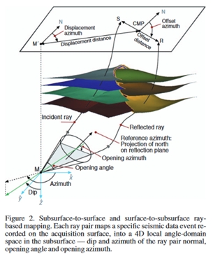
When we consider fractures, we look at the source-receiver azimuth as an important parameter. Using either the NMO velocity as a function of azimuth (low resolution) or the AVA as a function of azimuth (high resolution) we determine the orientation of the fracture system(s). But is this correct?
It might be, but not always. Namely, what is important is the local azimuth of the “incident ray” and the “reflected ray” at the reflection point, because they are directly influenced by the local fracture orientation at both sides of the interface. So, in case the “local azimuth” is significantly different from the surface source-receiver azimuth, it is important to consider it.
But how often does this occur? I think seldom, but yes in cases of complicated geology and stress fields. Now those occur often in places where significant hydrocarbons can be found and where drilling is very expensive: deep water with reservoirs below salt or basalt.
So, there are cases when considering the local angle domain (LAD) is a must for obtaining a correct image of the subsurface.
Geophysical Curiosity 7
A P-wave reflected by an interface will change in amplitude according to the reflection coefficient. Hence, when the acoustic impedance (ρvp) increases across the boundary, a positive amplitude (meaning the wavefront starts with a compression)
will remain a positive amplitude upon reflection.
But how about a S-wave? What will happen to the amplitude when reflected by an interface where the shear impedance (ρvs) increases?
The first thought would be that the reflection coefficient
will be positive, so the amplitude will keep the same polarity.
But, no, no, that is not the case. How confusing. Why can that be?
The answer lies in the fact that we use in the industry a moving reference frame.
So, for P waves, the positive direction is downwards on the way down and upwards on the way up.
What does this mean for S waves, say SH? It means on the way down the positive shear direction is to the right and on the way up the positive
shear is of course also to the right. But if the, say SH wave front start with a movement to the right and the shear impedance increases across the interface, on the way up the movement will be in the same direction. However, now that direction
is negative due to the choice of the frame we are using. So, the reflection coefficient is negative for an increase in shear impedance.
I hope it is no longer confusing.
Geophysical Curiosity 6
In Seismic processing often, the word “Stacking” is mentioned. Traditionally, stacking referred to applying an NMO correction to offset traces and adding them to form a stack trace, with improved signal-to-noise ratio.But do we still do stacking? Yes, we still do stacking, but in a different way. The stacking we do takes place in the imaging part of processing. Namely, in a modern processing scheme the data is prepared for imaging and after each offset is imaged, then the results are stacked. This can be most easily seen in case image gathers are built and displayed. After inspection and possibly re-imaging, these are the traces that are stacked.
Geophysical Curiosity 5
We are all aware of gravity, especially when you fall of your bike after too many drinks. Especially then it looks that gravity is a powerful force, although strictly speaking it is an acceleration. Interesting enough, gravity is the weakest force
in nature. How can that be? You would agree when you realize that it needs the whole earth, that is a mass of 6 1024 kg, to make me feel it. Also, according to Newton, if I meet another person, I should feel the “attraction” between
us, but I don’t. This shows how weak gravity is.
Geophysical Curiosity 4
“How confusing can you make it?” Take the description of anisotropy. The confusion is mainly due to using misleading symbols and different notations for the same quantities. Two examples: 1) using the symbol C for incompressibility and 2) the use of \( \delta \)(2) in one set of publications and \( \delta \)1 in other publications, both describing the same anisotropy parameter for propagation in the (x1,x3) plane. So, when reading publications make sure you are aware of the definitions.In describing wave propagation, the elastic and anisotropy parameters occur in the so-called stress-strain relationship which needs to be combined with Newton’s first law of motion to obtain the wave equation. In principle (“worst case”: triclinic symmetry) there are 21 different (C ij) parameters needed to describe the medium. Luckily in practice we can get away with fewer parameters and in the “best case” with only 2. For almost all practical applications we have the following cases: orthorhombic (7 Cij parameters), Transverse Isotropic (5 Cij parameters) and Isotropic (2 Cij parameters). Orthorhombic describes a finely layered medium with vertical fractures, Transverse Isotropic describes either fine layering or a set of vertical fractures only, whereas Isotropic describes a medium without any sub-seismic scale layering nor fractures.
For weak anisotropy, we use the following parameters:
Orthorhombic: Κ, \( \mu \), \( \epsilon \)(1), \( \epsilon \) (2), \( \delta \)(1), \( \delta \)(2) , \( \delta \)(3), \( \gamma \)(1), \( \gamma \)(2),
Transverse Isotropy: VTI: (Κ, \( \mu \), \( \epsilon \), \( \delta \), \( \gamma \)), HTI: (K, \( \mu \), \( \epsilon \)(v), \( \delta \)(v), \( \gamma \)(v))
Isotropy: K, \( \mu \)
Unhappily, all rocks should be considered triclinic, but in reality, we can “ignore” that. We wouldn’t be able to derive the needed 21 parameters from seismic observations anyway. So, let’s forget it and restrict ourselves to at most orthorhombic or tilted orthorhombic in case of dipping structures.
One quantity we can observe quite well with modern wide- or multi-azimuth acquisition and that is the orientation of fracture sets. Namely, the NMO velocity of waves travelling perpendicular to fractures is lower than waves travelling parallel to fractures. In addition, if S-waves can be observed (multi-component land or OBC acquisition) shear-wave splitting also indicates the orientation of fractures..
Geophysical Curiosity 3
“Keep it simple, you stupid” This slogan is of course based on the well-known political slogan “It’s the economy, you stupid” and here refers to “why introducing anisotropy parameters” in the description of wave propagation, given that
a full description of wave propagation is already complicated enough. The reason is that in general we don’t honour the real Earth when we try to model geophysical observations. In 1992, I gave an “oration” when I became Professor at the University
of Utrecht, called “Do we do justice to the Earth” with a wink to my wife’s occupation as a judge. It must be clear, that the title refers to all the approximation we make to make geophysical problems tractable. If we want to model exactly
the seismic response of real rocks, that means including small-scale inhomogeneities, we need complex mathematical algorithms and still can only do the modelling in detail for specific, well-described cases. And even then, you might wonder
whether in practice we know or even can use such detail.
It is exactly for that reason that effective media are used. In these media, the detail is “summarised/replaced” by “simple” anisotropy parameters. It might appear “making it
more complicated”, but after having familiarised yourself with it, you realize that it makes the description of wave propagation more realistic and especially more applicable. Nice examples are shown in the AVA exercise in the “Quantitative
Reservoir Characterization” course.
Geophysical Curiosity 2
We know that seismic energy can be propagated in the earth in two ways: P-waves and S-waves. Now in an isotropic elastic medium the P-wave particle displacement is in-line with the propagation direction and in case of an S-wave the particle displacement
is perpendicular to the propagation direction. This particle displacement can be in any direction as long as it is perpendicular to the propagation direction.
In anisotropic media, the situation is quite different.
For P-waves the particle displacement is deviating slightly from the propagation direction (ray direction), as the displacement is normal to the wave-front. The ray vector is namely no longer perpendicular to the wave-front.
For S-waves it is even more complicated. It was noticed in field experiments that the vertical S-wave reflection time from a horizontal interface differed depending on the polarization direction. Hence, the velocity did depend on the polarization.
Therefore, it was concluded that two S-wave modes exist, one with the particle displacement parallel (S-fast), the other with the particle displacement perpendicular (S-slow) to fracture orientation (or fine layering). In addition, the S-wave
can, and that is quite odd, only propagate with these two polarizations. So, if a source generates an S-wave with polarization in between, this S-wave will not propagate at all, but will split into the two
modes discussed before and each mode will propagate with its own velocity. This is called “shear-wave splitting” or “birefringence”. And again, the polarizations are not exactly perpendicular to the propagation direction. Instead, they are
perpendicular to the P-wave polarization, which as mentioned before, is neither in the propagation direction.
Geophysical Curiosity 1
When you look at the formula for the P-wave velocity, namely \( \sqrt[]{ \frac{K+4/3 \mu }{\rho}} \), with K the elastic modulus, which I rather call the stiffness or resistance to pure compression (only change in volume) and μ the resistance
to deformation (distortion without a change in volume), you realize that the P-wave is not a pure compressional wave. Pure compressional waves occur in media which have a shear modulus μ=0, such as water and air.
Please feel free to comment or add points of view and indicate whether you would like it to be mentioned on the website or not
(email: j.c.mondt@planet.nl).
© Breakaway