course news 31
Quantitative Seismic Interpretation
Doing
quantitative seismic interpretation, I experience that using Machine Learning
is a great way forward. However, an essential ingredient in many studies is to
use a rock physics model. For example, many relationships between elastic parameters
(IP, IS, density) and rock parameters (porosity and
permeability) are based on well logs with which we measure both sets of
parameters and can derive statistical relationships. But unfortunately, some
rock properties of interest are seldom measured in a well, such as anisotropy.
To predict rock properties from seismic with or without Machine learning, a
rock physics model is invoked. The model should be in some way be based on
relevant wells and then supplemented by an anisotropy component. Recent
publications show promising results. But note that to make progress a close
cooperation between the different disciplines in the geoscience is an essential
ingredient. Namely, without geological and petrophysical input it is impossible
to choose the right rock physics model, which is essential for the quantitative
interpretation of seismic data. I think we all agree in principle, but in practice the disciplines still tend to be active in silos.
My favourite exercise
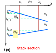
My favourite exercise is Time-Depth-Conversion using Raytracing. In this exercise we obtain insight into what a stacked or zero-offset section contains. Say we see on a (unmigrated) section two dipping events, and we want to convert these events to depth. This is equivalent to applying horizon migration or if we have uninterpreted seismic to full migration. But interesting is to realize that the time dips are a direct indication of the direction of emergence at the surface. Let us start with the upper horizon and surface location x1. The angle of emergence i1=arctan(V1.½Δt1/Δx), can be used as the angle of departure as it is zero-offset acquisition. Knowing the velocity, we can travel along this ray till travel time has been used up (maximum distance that can be travelled (t1,1 *v1). Doing this also for surface location x2 results in a second point on the reflector. As the reflection is a straight line, the reflector will also be a straight line. So, connecting these 2 depth points will result in the reflector.
But now the lower reflection. Again, as its arrival at the surface is in the upper velocity medium, we need to use that velocity to calculate its angle of emergence: i2=arctan(V1.½Δt2/Δx). Using this angle as angle of departure, we can ray trace in depth up to the first reflector, apply Snell’s law and determine the direction of travelling down below the first reflector. Doing it for the second surface location results in a second depth point on the reflector. Hence, we have both reflections converted to the two reflectors in depth.
Learning points:
1. What we see on a stack is the arrival direction of all reflections determined by the shallowest subsurface velocity (v1).
2. Each reflection can be down traced in the depth model using the established angle of departure and every time it encounters a reflector Snell’s law should be applied to establish in which direction to continue downwards to the next reflector.
Note the difference between reflection and reflector.
Classification scores: Is it a good idea to use the F1 score?
Is a harmonic mean always emphasizing the minimum of the precision and recall, hence does it always provide a pessimistic scoring of the models used for classification?
To evaluate the predictive power of a Machine Learning model cross-validation is used, separating the labelled instances into a training (80%) and a validation (20%) subset, where the separation is done randomly. The outcomes are:
True Positive (TP): the label is correctly predicted.
False Positive (FP): the predicted label is incorrect.
False Negative (FN): the label is not detected.
True Negative (TN): the correct label was not detected.
Precision = TP/(TP+FP): the fraction of True Positives among the detected class instances.
Recall = TP/(TP+FN): the number of True Positives over the number of class instances detected.
The question now is: Is it better to have a high Precision or a high Recall (Sensitivity)?
Obviously, the best is to have both, and the worst is to have a model with a poor precision and a poor recall, no doubt. But what if one is good and one is poor? Could we average the two values?
Let’s do it and let’s try two kinds of averaging:
Considering Precision and Recall are values between 0 and 100%, the two types of mean can be displayed using the same colour code for means between 0 and 100 for all the values of P and R:
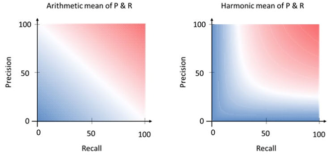
We can see on the graphic above that the harmonic mean will be high (red) only if both (P and R) are high and will be low (blue) as soon as one of the two is low. This is not the case with the arithmetic mean where a mean of 50 (white) may be obtained if one of the two is null and the second = 100.
Imagine now a COVID test which always replies ‘positive’ for any test and let’s apply this test on 100 people, 5 being affected, 95 being healthy, hence TP = 5, FP = 95, FN = 0, Precision = 5 / (5+95) = 5%
·and Recall = 5 / (5 + 0) = 100%. We can now compare the two means we have considered above:
A = Arithmetic mean = (5 + 100) / 2 = 52.5% and H = Harmonic mean = 2*5*100/ (100+5) = 9.5%
It is clear the harmonic mean is better to say this covid test is poor! This harmonic mean is called F1.
OK, but now, another criticism may raise up: The F1 score give an equal importance to the Recall or to the Precision and in some cases I may be more interested by one of the two. In fact, the F1 scoring is just a specific case of the Fβ score defined as:
Fβ=(1+β2) *(P*R/[(β2*P) +R]
If it is needed to make an emphasis on the Precision, it is possible to replace the F1 score by a F ½ score. For the poor COVID test seen above, the F ½ value will be F ½ = (1+ 1/4) * 5 * 100/ (((1/4) *5) +100) = 625 / 101.25 = 6.17. Hence, F ½ is more sensitive to precision.
In case it is necessary to detect more class instances from a data set and we are tolerant to some false positive values, it may be recommended to replace the F1 by F2. For the COVID test above:
F2 = (1+4) *5*100 / ((4*5) +100) = 2500 / 120 = 20.83. Hence, F2 is more sensitive to Recall.
Reference: Henri Bondelle, Force
Can I restrict the input of ChatGPT to dedicated websites?
I wanted to see whether it is possible to limit the input for ChatGPT to a single website. I used my own website as you can see below. Unfortunately, it is not possible to restrict the ChatGPT input to a single or multiple websites.

Another interesting
experiment with ChatGPT.
You can use a wide range of languages, but it is interesting to notice that the answers are different, that is they are not a direct translation. The English version seems to be the most complete. See below for an example:
What is Geophysics?
Geophysics is a branch of Earth science that focuses on the study of the Earth's physical properties and the processes that affect it. It involves the application of principles and methods from physics to understand the Earth's structure, composition, and behavior, both on the surface and in its interior. Geophysicists use various techniques and instruments to gather data about the Earth and interpret that data to gain insights into its geological, environmental, and geodynamic processes.
Some key areas of study within geophysics include:
1. **Seismology**: This field involves the study of seismic waves generated by earthquakes, explosions, or other sources. Seismologists use this data to understand the Earth's internal structure and monitor seismic activity.
2. **Geomagnetism**: Geomagnetists study the Earth's magnetic field and its variations over time. This field is essential for understanding the Earth's magnetic properties and how they relate to geologic processes.
3. **Gravity and Gravimetry**: Gravity surveys and measurements help geophysicists map variations in the Earth's gravitational field. These variations can provide information about subsurface geology and density variations.
4. **Geoelectrics**: Geoelectric methods involve measuring the electrical properties of rocks and sediments to map subsurface structures and groundwater resources.
5. **Ground Penetrating Radar (GPR)**: GPR uses radar pulses to image the subsurface and is commonly used for archaeological and engineering purposes.
6. **Remote Sensing**: This involves using satellite-based and aerial instruments to collect data on the Earth's surface, including its topography, temperature, and vegetation cover.
7. **Exploration Geophysics**: In the context of resource exploration (such as oil, gas, minerals, and groundwater), geophysics is used to locate and assess the extent of subsurface resources.
8. **Environmental Geophysics**: Geophysics is also used to study environmental issues, such as monitoring groundwater contamination, assessing the stability of dams and levees, and investigating geological hazards.
9. **Planetary Geophysics**: Geophysical techniques are applied to study other celestial bodies, such as planets, moons, and asteroids, to understand their composition and internal processes.
Geophysicists play a crucial role in various fields, including natural disaster monitoring and mitigation, resource exploration, environmental protection, and understanding the Earth's geological history. Their work often involves collecting data through field surveys, laboratory experiments, and computer modelling to advance our knowledge of the Earth's physical properties and processes.
Qu’est-ce qu’est Géophysique ?
La géophysique est une branche des sciences de la Terre qui se concentre sur l'étude des propriétés physiques de la Terre et des phénomènes géologiques en utilisant des méthodes de mesure et d'analyse physiques. Elle vise à comprendre la structure interne de la Terre, son comportement dynamique, et les processus qui se produisent à l'intérieur et à la surface de la planète.
Les géophysiciens utilisent une variété de techniques et d'instruments pour recueillir des données sur la Terre, notamment la sismologie (étude des ondes sismiques pour comprendre la structure de la croûte terrestre et surveiller les tremblements de terre), la géodésie (mesure de la forme et de la gravité de la Terre), la magnétométrie (étude des variations du champ magnétique terrestre), la gravimétrie (mesure des variations de la gravité), la géothermie (étude de la chaleur interne de la Terre), et d'autres techniques.
Les informations obtenues grâce à la géophysique sont essentielles pour divers domaines, notamment la prospection pétrolière et gazière, l'exploration minière, la prévision des risques naturels (tels que les tremblements de terre et les volcans), la compréhension des processus tectoniques, et la recherche sur le climat et l'environnement. En résumé, la géophysique est une discipline clé pour mieux comprendre la planète sur laquelle nous vivons.
Wat is geofysica?
Geofysica is een wetenschappelijke discipline die zich bezighoudt met het bestuderen van de fysische eigenschappen en processen van de aarde en andere hemellichamen in het heelal. In het Nederlands wordt geofysica soms ook wel "aardfysica" genoemd. Het is een interdisciplinair vakgebied dat elementen van de geologie, natuurkunde en wiskunde combineert om fenomenen zoals seismologie, geothermie, zwaartekracht, magnetisme, elektriciteit en andere fysische aspecten van de aarde te onderzoeken. Geofysica wordt vaak toegepast om inzicht te krijgen in de structuur en processen van de aarde, bijvoorbeeld bij het bestuderen van aardbevingen, vulkanen, grondwaterstromen en andere geologische verschijnselen.
Use of OpenAI in Google
It is very helpful to add OpenAI to Google. You only need a Google account, which you have having a gmail account.When making exercises in Google Colab, I found it very helpful to use OpenAI to get some additional information on a method or to solve some of the coding issues often occurring when trying to apply an existing code to my own dataset.For coding issues, I keep my exercise in one window and in another window, I paste the error message. OpenAI will then suggest a solution, which otherwise I must search for on many websites.
Example I:
The Google Colab error message:
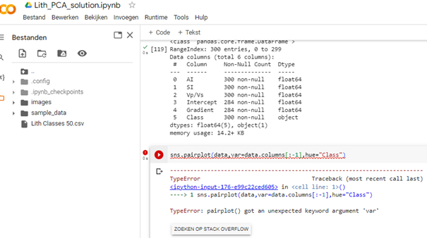
ChatGPT help message:
The error you're encountering is due to the fact that you are trying to access a non-existent attribute called 'column' in a pandas DataFrame object. It seems like you're attempting to use this attribute to specify the columns of your DataFrame for the pairplot. However, the correct attribute to use is 'columns' (plural), not 'column' (singular).
Here's the corrected version of your code:
sns.pairplot(data, vars=data.columns[:-1], hue="Class")
In this code, data.columns returns a list of all column names in your DataFrame, and data.columns[:-1] slices the list to exclude the last column, which seems to be used as the target or class column. This updated code should work without any attribute errors.
Example II:
Question Can Principal Component Analysis be used for Feature Selection?
ChatGPT: Principal Component Analysis (PCA) is primarily a dimensionality reduction technique, not a feature selection technique. However, it can indirectly help with feature selection in certain cases.PCA works by transforming the original features into a new set of orthogonal (uncorrelated) features, called principal components. These components are ordered in such a way that the first component captures the most variance in the data, the second component captures the second most variance, and so on. By selecting a subset of these principal components, you can effectively reduce the dimensionality of your data.
While PCA itself doesn't perform explicit feature selection, it can still help in the following ways:
1. Reducing Dimensionality: By selecting only the first few principal components that capture most of the variance in the data, you effectively discard less informative dimensions and retain the most important aspects of the data.
2. Noise Reduction: PCA can help in removing noise and irrelevant variations in the data, leading to better generalization and potentially improved model performance.
3. Visualizing Data: PCA can be used to visualize high-dimensional data in a lower-dimensional space (usually 2D or 3D), making it easier to identify patterns, clusters, or outliers.
4. Simplifying Model Complexity: Using a reduced set of principal components as input features to a machine learning model can simplify the model's complexity and potentially improve its efficiency.
However, PCA does not inherently consider the relationships between the original features and the target variable. If you're interested in feature selection that takes the target variable into account, you might consider other techniques such as:
1. Univariate Feature Selection: Methods like chi-squared test, mutual information, or F-test can be used to select features based on their individual relevance to the target variable.
2. Recursive Feature Elimination (RFE): This is an iterative method that starts with all features and eliminates the least important features in each iteration based on a chosen model's performance.
3. Lasso Regression: Lasso (Least Absolute Shrinkage and Selection Operator) is a regularization technique that can lead to automatic feature selection by shrinking the coefficients of less important features to zero.
4. Tree-based Methods: Decision trees and random forests can provide feature importances that you can use for feature selection.
Remember that the choice of feature selection technique depends on the nature of your data, your goals, and the specific machine learning algorithms you intend to use. Sometimes, a combination of techniques might yield the best results.
Comparison of 3 ChatGPT's
There are several ways of using Large language Models. I have compared the answers to a simple question: “What geophysical methods are available”, using ChatGTP3, ChatGPT4 and BingChatGPT. Instead of ChatGPT4 I was linked with ChatGPT3.5.
I have the following comments:
ChatGTP3
The answer was quite comprehensive. Only surface and Scholte waves were missing under seismic. MT should have been mentioned explicitly under Electrical or Magnetic methods. Hyperspectral imaging under remote sensing includes radiometric surveys.
ChatGPT3.5
The answer is far from complete: gravity, remote sensing and GPR are not mentioned. Interesting is that the sources of information are explicitly mentioned (with links).
Bing ChatGPT
The answer is based on Wikipedia and the US Environmental Protection Agency. It provided the least information. Note that Bing AI has additional features that ChatGPT does not have, such as the use of images, which I haven’t tried.
My conclusion: I will use for the time being ChatGPT3 in my courses.
The full answers are given below.
ChatGTP3:Q: What geophysical methods are available?
A: Geophysical methods are techniques used to study the Earth's subsurface and understand its physical properties. There are numerous geophysical methods available, each with its own principles and applications. Here are some commonly used geophysical methods:
1. Seismic methods: Seismic techniques involve generating and recording waves that propagate through the subsurface. These waves can be either compressional (P-waves) or shear (S-waves). Seismic methods include:
o Reflection Seismic: Used to image subsurface structures and identify potential hydrocarbon reservoirs or geological formations.
o Refraction Seismic: Measures the travel times and velocities of seismic waves to infer subsurface layering and geologic boundaries.
o Seismic Tomography: Provides detailed information on subsurface velocity variations, used for imaging complex structures.
2. Electrical methods: Electrical methods measure the electrical properties of the subsurface materials. These methods include:
o Electrical Resistivity Tomography (ERT): Measures the subsurface resistivity distribution, useful for mapping geologic features and groundwater studies.
o Induced Polarization (IP): Measures the ability of rocks to hold an electric charge, used for mineral exploration and detecting subsurface sulfide minerals.
3. Ground Penetrating Radar (GPR): Uses high-frequency electromagnetic waves to image the subsurface. It is effective for locating buried objects, mapping shallow geologic structures, and assessing pavement conditions.
4. Magnetic methods: Magnetic methods measure the Earth's magnetic field variations caused by subsurface materials. They include:
o Magnetic surveys: Used for mapping subsurface structures, identifying mineral deposits, and detecting buried ferrous objects.
o Magnetic gradiometry: Measures the spatial variation of the magnetic field, providing more detailed information about subsurface features.
5. Gravity methods: Gravity surveys measure variations in the Earth's gravitational field caused by variations in subsurface density. These surveys are valuable for mapping large-scale subsurface structures, such as sedimentary basins or fault zones.
6. Remote Sensing: Although not strictly a geophysical method, remote sensing uses satellite or airborne sensors to collect data about the Earth's surface. Techniques such as LiDAR (Light Detection and Ranging) and hyperspectral imaging provide valuable information for geological and environmental studies.
These are just a few examples of geophysical methods available. Each method has its strengths and limitations, and the choice of method depends on the specific objectives and characteristics of the subsurface being investigated.
ChatGPT4
Q: What geophysical methods are available?
A: Reading webpages...
There are several geophysical methods available for subsurface investigations. Some of the commonly used methods include:
1. Magnetic surveys: Measure variations in the Earth's magnetic field to identify magnetic minerals and geological structures.
2. Electromagnetic (EM) surveys: Induce an electromagnetic current into the ground and measure the resulting field to detect changes in conductivity, which can indicate the presence of geological features or mineralization.
3. Resistivity surveys: Measure the electrical resistance of the subsurface to identify variations in rock types, groundwater, and potential mineralization.
4. Induced Polarization (IP) surveys: Measure the decay of voltage over time to assess the chargeability of rocks, which can indicate the presence of mineral deposits.
5. Seismic surveys: Generate and record seismic waves to image subsurface structures and identify geological boundaries.
6. Radiometric surveys: Measure natural radiation levels to identify radioactive minerals and map rock types.
These methods can be used individually or in combination to provide a comprehensive understanding of the subsurface geology and potential mineral resources. The selection of the appropriate method depends on the specific objectives of the study and the geological conditions of the area.
Source
Geophysical Methods, Exploration Geophysics » Geology Science
Geophysical Method - an overview | ScienceDirect Topics
Geophysical Methods - Enviro Wiki
Bing ChatGPT
Q: Which geophysical methods are available
A: Geophysical methods are techniques that apply various principles of physics to investigate the physical properties of the subsurface. According to Wikipedia1, geophysical methods can be classified into solid earth applications and fluid dynamics applications. Solid earth applications include studying the Earth’s shape, gravity, magnetic, and electromagnetic fields, its internal structure and composition, its dynamics and plate tectonics, and its volcanism and rock formation. Fluid dynamics applications include studying the water cycle, the oceans and the atmosphere, the ionosphere and magnetosphere, and the solar-terrestrial physics.
According to the US Environmental Protection Agency2, geophysical methods can also be categorized by the environment in which they are applied: on the earth surface, within a borehole/well, or on a surface waterbody. Some examples of commonly employed geophysical methods are:
- Surface geophysical methods: seismic reflection and refraction, gravity, magnetic, electrical resistivity, electromagnetic induction, ground-penetrating radar, etc.
- Borehole geophysical methods: acoustic televiewer, caliper, density, fluid conductivity and temperature, gamma ray, magnetic susceptibility, neutron porosity, etc.
- Waterborne geophysical methods: bathymetry, side-scan sonar, sub-bottom profiling, marine magnetometer, etc.
I hope this helps you understand what geophysical methods are available. 😊
ChatGPT
Huge attention is being paid to the use of Artificial Intelligence in education, especially since ChatGPT has been introduced by OpenAI. The question is how beneficial and/or detrimental it is with respect to the creativity of students and course participants.
I have decided that it should be embraced in my courses as I see great benefits. Below is an example of the answer that ChatGPT gives to a simple question. Finding the answer, yourself searching websites takes a lot of time. Although the answer might be considered not very specific/detailed, that means quantitative, it still provides a good starting point for further digression.
Question: Which method has better resolution gravity, magnetics, electromagnetics, seismic?
Answer ChatGPT
The resolution of geophysical methods can vary depending on several factors, including the properties of the subsurface, the survey design, and the data processing techniques employed. In general, it is challenging to determine a definitive ranking for resolution between different geophysical methods, as their effectiveness can vary depending on the specific application and geological conditions. However, I can provide a general overview of the resolution capabilities of the methods you mentioned:
1. Gravity: Gravity surveys measure variations in gravitational acceleration caused by variations in subsurface density. Gravity data can provide information about large-scale features and density contrasts in the subsurface. However, gravity surveys typically have lower resolution compared to other methods, as they are more sensitive to larger and deeper structures rather than small-scale features.
2. Magnetics: Magnetic surveys detect variations in the Earth's magnetic field caused by magnetic properties of the subsurface. They are effective in identifying magnetic anomalies associated with certain geological structures, such as mineral deposits or igneous intrusions. Magnetic surveys can provide good resolution for mapping shallow structures, but their effectiveness decreases with depth.
3. Electromagnetics: Electromagnetic (EM) methods involve the measurement of electromagnetic fields to investigate subsurface conductivity variations. EM surveys are sensitive to the presence of conductive materials, such as minerals or fluids. They can provide high resolution, especially for mapping shallow targets or near-surface features. However, their effectiveness diminishes with depth, and the resolution can be influenced by factors like survey frequency and target conductivity.
4. Seismic: Seismic surveys use sound waves (generated artificially or by natural sources) to image subsurface structures and rock properties. Seismic data can provide excellent resolution, particularly for imaging geological structures, stratigraphy, and fluid reservoirs. The resolution of seismic methods can vary depending on factors like wave frequency, source-receiver configuration, and subsurface conditions. High-frequency seismic waves generally offer better resolution for shallow targets, while lower frequencies are suitable for deeper investigations.
It's important to note that the choice of method depends on the specific objectives of the survey, the geological setting, and other practical considerations. Often, a combination of multiple methods is employed to improve subsurface imaging and interpretation.
Question: Which outstanding developments have taken place in quantitative Reservoir Characterisation since 2022?
Answer ChatGPT
As an AI language model, my knowledge is based on data up until September 2021, so I might not be aware of the specific developments in quantitative reservoir characterization that have taken place since 2022. However, I can provide you with an overview of some general advancements that have been observed in this field in recent years. It's important to note that there may have been additional advancements beyond my knowledge cutoff date.
1. Machine Learning and Artificial Intelligence: The application of machine learning and artificial intelligence techniques has significantly advanced reservoir characterization. These technologies help analyze large datasets, integrate multiple data sources, and improve predictions and interpretations.
2. Advanced Seismic Imaging: Developments in seismic imaging have enhanced reservoir characterization by improving the resolution and quality of subsurface images. Techniques such as full-waveform inversion, reverse time migration, and multi-component seismic imaging have contributed to more accurate subsurface mapping.
3. Advanced Petrophysical Analysis: Petrophysical analysis techniques have evolved to provide more accurate and detailed information about reservoir properties. Advanced well logging tools, such as nuclear magnetic resonance (NMR) and dielectric logging, enable improved characterization of petrophysical properties, fluid saturation, and rock typing.
4. Data Integration and Multidisciplinary Approaches: Reservoir characterization has seen advancements in integrating various types of data, including well logs, seismic data, production data, and geological models. Multidisciplinary approaches that combine geological, geophysical, and engineering data provide a more comprehensive understanding of reservoir properties and behavior.
5. Reservoir Simulation and Optimization: Advanced reservoir simulation techniques have become more sophisticated, allowing for more accurate modeling and prediction of reservoir performance. Coupled with optimization algorithms, these simulations help optimize reservoir management strategies and improve recovery efficiency.
6. Data-Driven Models and Uncertainty Quantification: The use of data-driven models, such as machine learning algorithms and data assimilation techniques, has gained prominence in reservoir characterization. These models can handle large datasets, capture complex relationships, and provide insights into uncertainty quantification, leading to more robust reservoir characterizations.
It's important to consult the latest research papers, industry publications, and attend conferences or seminars to stay up to date with the most recent developments in quantitative reservoir characterization since 2022.
Conclusion: The latest developments are unknown to ChatGPT. Another reason to follow my courses.
A new philosophy in seismic processing an imaging
The conventional processing sequence looks like:
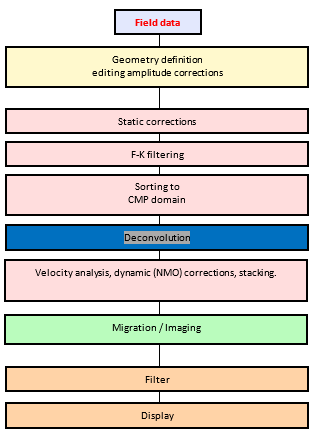
The
core of the sequence is migration or imaging of the data. But, to comply with
the assumptions of the conventional imaging algorithm: the data set should consist
of primary reflections only. This means that extensive pre-processing is
needed. The signal-to-noise ratio should be improved, multiples to be removed,
etc. For each pre-processing step parameters need to be tested before application.
This requires extensive human interaction.
Is there a solution? Yes. The solution is to use multi-parameter
Full Waveform Inversion and Imaging. FWI imaging is a least-squares
multi-scattering algorithm that uses raw field data (transmitted and reflected arrivals
as well as their multiples and ghosts) to determine many different subsurface
parameters: velocity, reflectivity, etc. Also, anisotropy of the subsurface can
be determined.
The new processing sequence looks like:
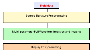
Note,
only the source signature is needed, derived from near-field hydrophones, which
can be refined by shot least-squares direct arrival inversion in FWI matching
modelled and observed data.
The conclusion of the authors: It would be remiss of us not
to ask whether it is time to set aside the old subjective workflow of pre-processing,
model building and imaging and instead embrace a new era of seismic imaging
directly from raw field data? (Ref: McLeman et al, The Leading Edge, 2022, N1.)
This approach will be part of my course “Advanced Seismic Acquisition
& Processing”.
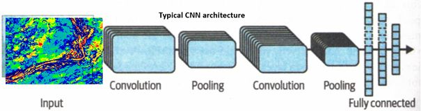
Pooling
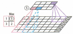
The aim of pooling is to reduce the input image in order to reduce the compute load. Each neuron in a pooling layer is connected to a limited number of neurons in the preceding layer, located within a small rectangular area (see figure on the left). A pooling neuron does not use connection weights, just combines the values in the area according to specification: average or maximum. In the figure only the maximum in the 2x2 area makes it to the next layer. Also a stride of 2 is used, reducing output image by a factor 4. (No padding at the edges).
Pooling is usually done between the convolutional layers and
is applied to all the outputs of the convolutional filters.
Reference: Hands-on Machine Learning with
Scikit_Learn, Keras & TensorFlow by Aurélien Géron
In Machine Learning 2 techniques are of great importance: Dropout and Transfer Learning. Dropout was discussed under Geophysical curiosities, here we will dicuss Transfer learning.
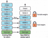
In the future software companies will offer for sale trained Deep Learning Networks for specific tasks like seismic interpretation, reservoir characterization, etc. These DNN’s, although trained on specific data sets are a good starting point for building your own models/algorithms for your data, as training from scratch requires a large and expensive compute effort. Those models are based on relevant but still different training instances, thus how do I adapt the model for my own data? The technique is called “Transfer Learning”.In Transfer Learning you take an existing DNN trained for a task A (shown on the left) and freeze the lower layers, as they will handle the most basic characteristics of for example a picture and only replace a few upper hidden layers with new to be trained layers for your task B (shown on the right). The more similar the tasks the fewer layers need to be retrained. For a very similar task only the output layer needs to be replaced.Train your new model on your dataset and evaluate its performance. Then unfreeze the upper frozen layers, so that the training can also tweak the hyper parameters. This will improve the performance without demanding extensive compute time.
Reference: Hands-on Machine learning with Scikit_Learn, Keras & TensorFlow, Aurélien Géron
Course News 20
In my Machine Learning courses I have used so far, the open-source package Weka. The reason is that it is a user-friendly and easy to run package with most relevant Machine learning algorithms, except truly Deep Learning. This suffices for most exploratory applications, where we like to learn the workflows and applications of Machine learning. Weka also has an option to build your own sequence (KnowledgeFlow) in such a way that data is not stored in memory and therefore allows applications to very large data sets. A disadvantage of Weka is that deep learning can be done with only one hidden layer, but in practice it takes too long using a CPU.
Therefore, I have included in my courses an introduction to Google Colab. This runs on the Cloud and allows use of a GPU or a TPU. It is “the way” to learn using a whole range of open-source Machine Learning algorithms. In an exercise you get acquainted with using interactive python notebooks, how to get algorithms using sklearn and if you restrain yourself from using it in earnest on large datasets, it is free.
Course News 19
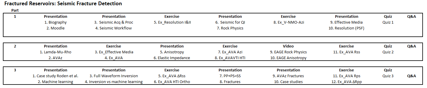
As part of a more extensive course on Fractured Reservoirs, I have developed the geophysical part called "Seismic Fracture Detection". It discusses the seismic acquisition requirements for multi-azimuth analysis using NMO velocity anisotrop one way to determine the fracture orientation of vertical fracture systems and Amplitude versus Angle of Incidence for more resolution and determination of fracture densisty.. P-wave, PS wave or Converted wave and S-wave data are discussed and used in AVA exercises. The program, which could be fully interactive, is as follows:
Course News 18
Compressive sensing, a method with which significant savings in acquisition costs can be achieved, is getting more and more attention as 3D surveys get bigger and continuous monitoring is used more often, also for CO2 storage and geothermal.
Compressive sensing circumvents the Shannon-Nyquist criterium of taking 2 samples per wavelength. It utilises sparsity of data in a transform domain, for example Fourier or Radon domain.
The crux of the method is that the data / wavefield will be on purpose (lower cost) under-sampled, but the resulting sampling (aliased) noise can be “filtered out / removed / suppressed” at the benefit of the needed data / wavefield. This allows the reconstruction of the wavefield in the state it would be acquired using full Shannon-Nyquist sampling. There are a few assumptions, however: there must exist a transform domain where the data is sparse, and the necessary random sampling must include the sampling of the desired reconstructed wavefield.
The topic has been added to the Advanced Seismic Data Acquisition and Processing courseCourse News 17
I have built two short courses of importance to the "Energy Transition". The first one is called "Geophysics for Geothermal Energy" and deals with the two most relevant geophysical technologies: seismic and Electromagnetic (EM) methods. The second one is called "Geophysics for CO2 sequestration and Enhanced Oil Recovery (EOR)". This course includes the use of Gravity and Gravity Gradiometry, in addition to Seismic and ElectroMagnetism, to monitor the CO2. Both courses are 2-day courses, with presentations, exercises and quizes to reenforce the learning. As with all my courses, they can be followed interactively, using Moodle, or Face-to-Face (F2F). They also can be combined or made part of a package of Transition relevant EPTS courses.


Course News 16
In the past we always talked about Seismic and Non-Seismic methods. But I was never quite happy with the indication Non-Seismic. An equivalent issue exists with the name Vertical Transverse Isotropy. It would be better to call it Polar Anisotropy, as that name directly refers to the relevant property, namely anisotropy. Therefore, I am pleased by the increasing use of the word Multi-Physics instead of Non-Seismic. This directly indicates the use of many different (geo)physical measurements used (gravity, magnetics, electromagnetics, self-potential, etc and seismic). In due time I will replace Non-seismic by Multi-Physics in my courses.
Course News 15
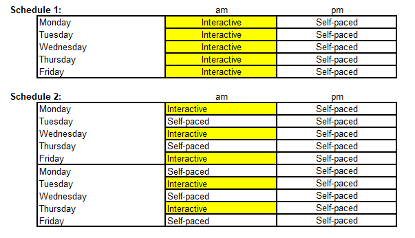
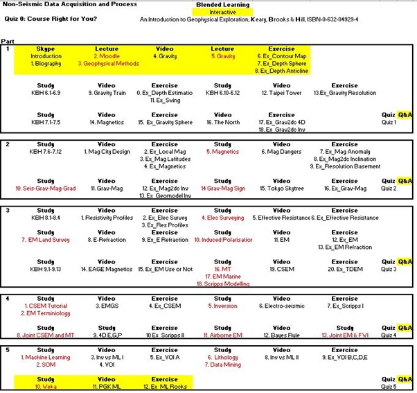
From recent experience with Blended Learning courses, I have decided to increase the interactive parts of the course. In a 5-day course, I will have each day a half day interactive session and the other half will be self-paced reading and doing the exercises. Below an example of the new schedule for the Non-Seismic Data Acquisition and Processing course. All other courses will be updated similarly.
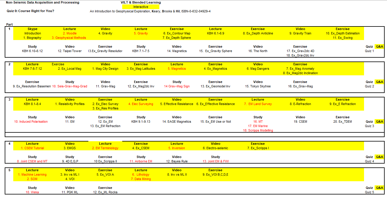
For all my Blended Learning courses, consisting of 5-parts (equivalent to a 5-day F2F course) a choice can be made between the following two schedules:
Course News 14
Part 1:
Day 1: 3 hours interactive presentation & discussion,
Day 1&2: 4 hours self-paced exercises+learning-reinforcement quiz 1
Part 2:
Day 3: 3 hours interactive presentations & discussion
Day 3&4: 4 hours self-paced exercises+learning-reinforcement quiz 2
Part 3:
Day 4: 3 hours interactive presentation & discussion,
Day 4&5: 4 hours self-paced exercises+learning-reinforcement quiz 3
Part 4:
Day 5: 3 hours interactive presentations & discussion
Day 5&6: 4 hours self-paced exercises+learning-reinforcement quiz 4
Part 5:
Day 7: 3 hours interactive presentation & discussion,
Day 7&8: 4 hours self-paced exercises+learning-reinforcement quiz 5
Course News 13
The main reason is that as it is a E-Learning, self-paced course the client can adapt the time schedule (say, when staff also must work half days).
Two examples of the alternatives:
Machine Learning for Geophysical Applications (MLGA)Day 1: 3 hours interactive presentation & discussion
Day 1&2: 4 hours self-paced exercises+learning-reinforcement quiz 1
Part 2
Day 3: 3 hours interactive presentations & discussion
Day 3&4: 4 hours self-paced exercises+learning-reinforcement quiz 2
Part 1
Day 1: 3 hours interactive presentation & discussion,
Day 1&2: 4 hours self-paced exercises+learning-reinforcement quiz 1
Part 2
Day 3: 3 hours interactive presentations & discussion
Day 3&4: 4 hours self-paced exercises+learning-reinforcement quiz 2
Part 3
Day 4: 3 hours interactive presentation & discussion,
Day 4&5: 4 hours self-paced exercises+learning-reinforcement quiz 3
Part 4
Day 5: 3 hours interactive presentations & discussion
Day 5&6: 4 hours self-paced exercises+learning-reinforcement quiz 4
Part 5
Day 7: 3 hours interactive presentation & discussion,
Day 7&8: 4 hours self-paced exercises+learning-reinforcement quiz 5
Course News 12
The change in reflection strength with increasing angle of incidence (AVA) can provide important information with respect to the properties of reservoirs. Although formulations exist for strong contrasts across an interface, weak contrasts are more common in sedimentary sequences. This leads to formulations, through linearization, which provides insight in the influence of the elastic parameters across the interface on the AVA behaviour. These expressions can also be extended to include anisotropy of the media and in case of weak anisotropy the expressions still allow insight into the influence of the anisotropy contrasts across the interface on the AVA behaviour.
An interesting question is: Can we express the AVA behaviour in terms of the isotropic expressions using generalised elastic properties?
The answer is yes, we can with so-called pseudo-elastic properties. These are function of the true elastic properties modified by expressions involving the anisotropy parameters.
An example for VTI:
with
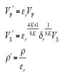
The use of pseudo-isotropic parameters is added to the Quantitative Reservoir Characterisation Blended Learning and F2F Course.
Course News 11
A new short course has been developed on the use of Machine Learning for prediction of facies along a borehole. Based on a reasonable number of interpreted wells various algorithms can be compared in classifying wellbore profiles of “new” unlabelled wells. In the course it will be shown that limited training data (1 well) results in poorer predictions than when more labelled data can be used for training. It also is found that using a Deep Neural Net results in the best classification. In addition, the use of semi-supervised learning, often needed in geoscience applications because of limited availability of labelled data, is discussed. The course is available in a Face-to-Face and an E-learning version.
Course News 10
I am happy to announce that I have been officially nominated as short course instructor with the EAGE.
Course News 9
To each course a multiple-choice quiz has been added. The aim is not only to provide a test of what has been learned but also as a way of enhancing the participants understanding of the subjects.
Course News 8
Based on Open Source software, a one-day (8hrs) Face-to-Face and a one-month duration (8hrs equivalent) E-learning course called “Introduction to Machine Learning for Geophysics” have been developed. Both courses contain power point presentations with references to publications together with computer-based exercises and Machine Learning related videos.
The exercises deal with a genuine geophysical issue, namely predicting lithology and pore fluids, including fluid saturations. The input features are Acoustic and Shear Impedances, Vp/Vs ratios and AVA Intercept and Gradients. Several exercises deal with pre-conditioning the datasets (balancing the input categories/instances, standardization & normalization of features, etc), the others apply several methods to classify the “instances” (Machine Learning terminology for cases): Bayes, Logistic, Multilayer Perceptron, Support Vector, Nearest Neighbour, AdaBoost, Trees, etc. This for supervised and unsupervised applications. Also, non-linear Regression is used to predict fluid saturations
Course News 7
July 24th 2019
Update on Machine Learning courses for Geophysics
Based on Open Source software I have developed a one-day (8hrs) Face-to-Face and a one-month duration (8hrs equivalent) E-learning course called “Introduction to Machine
Learning for Geophysics”. These courses are made up of power point presentations with references to publications together with computer-based exercises and Machine Learning related videos.
Course News 6
June 4th 2019
Machine Learning
Based on Open Source software I have developed an “Introduction to Machine Learning” together with computer-based exercises. The Introduction will be included in all my courses, but the exercises will be
topic specific. Apart from the Face-to-Face / Classroom courses I plan to develop very short E-learning courses (the equivalent of a one-day course) on the use of Machine Learning in Basic Geophysical Data Acquisition and Processing, Advanced
Seismic Acquisition/Processing/Interpretation, Quantitative Reservoir Characterization and Non-Seismic Data Acquisition and Processing.
Course News 5
Feb. 20th 2019
Course News 4
Dec. 24th 2018
In the courses the new approach of “Machine Learning” will be included. First in the form of lectures, followed later by exercises. Machine learning, also defined as Artificial Intelligence or Algorithms, relate to the use of statistical methods
to derive from large (learning) data sets relationships (“correlations”) between observations and subsurface properties, for example lithological facies or fluid saturations.
This is a clear break with the traditional approach in
which we ‘totally’ rely on understanding the physics of the subsurface processes (say visco-acoustic wave propagation) causing the observations or data (amplitude anomaly) at the surface.
In Machine Learning we mimic human “brain
processes” to learn from a very large number of labelled cases how to explain a new case. In analogy with when you have seen more cases, had a longer learning trajectory, you are better able to evaluate a new case. You might not fully
understand why events happen, but you have learnt how to deal with them, i.e. you can classify them say as beneficial or threatening.
Course News 3
Aug. 17th 2018
In the “Advanced Seismic Data Acquisition and Processing” Course two new topics have been introduced: 1) Blended acquisition and 2) Penta-source acquisition.In blended acquisition sources are fired closely in time such that the records do overlap. To separate the responses of the subsurface two methods can be applied.
One method is called “dithering” in which a “random” variation is applied to the auxiliary sources with the result that their responses are non-coherent and can be considered as random noise and be removed/suppressed in processing. As the “dithering” for each auxiliary source is known, it can be removed resulting in coherent records for each, leaving the other source records incoherent.
The other method uses “seismic apparition”. In this method a periodic variation, be it time delay or amplitude scaling, is applied to each source and each source response can be made to “appear” at the expense of the responses of the other sources this is often done in the KF domain.
The Penta-source (Polarcus), consists of 6 arrays (spaced 12.5 m apart), which are used in more than one source configuration resulting in 5 single sources. For operational reasons they are fired in the following sequence: (1,2), (3,4), (5,6), (2,3), (4,5). They can be used with a shot-point interval of 12.5 m and “dithered” over 1 s, or with a shot interval of 62.5 m and “dithered” over 5 ms, allowing deblending of the shot records. Note that the first part (1 or 5 s) of the record is “clean” and do not require deblending.
In both cases also the streamer spacing might vary, where an increasing separation from centre spread outwards is beneficial for a high-resolution shallow image.
Course News 2
In addition to the “Effective Media and Anisotropy” an extensive AVA modelling exercise has been implemented. It allows investigating the various aspects of AVA analysis, namely what rock and fluid properties can be derived from observing
the Amplitude changes with Angle of incidence on the interface between two rocks. It not only deals with density, P- and S-wave velocities, but also with anisotropy. From the anisotropy, not only average properties of sub-seismic-scale
fine layering, but maybe even more important fracture orientation and density can be derived. These are important in relation to where to drill production wells relative to injection wells (think of fractured carbonates).
In the
exercise the AVA response of different rock interfaces (shale, sand, salt, limestone, etc) can be modelled using Vertical Transvers Isotropy (VTI) for fine layering and Horizontal Transvers Isotropy (HTI) related to fractures. Although
more than one fracture set do occur in nature, the exercise is limited to one fracture set, based on the idea that most often it is the present stress regime that keeps fractures open in the minimum horizontal stress direction.
Course News 1
For the “Quantitative Reservoir Characterisation” (QRC) course a new module has been designed concerning Effective Media and Anisotropy. The Earth is often too complicated in terms of inhomogeneities to fully honour it in modelling wave propagation and inversion. The solution has been to replace the real earth by a so-called effective medium. This effective medium allows an “appropriate approximation” of the wave propagation and inversion. Although an approximation, it is still appropriate for solving the issue at hand.One main application is related to the concept of anisotropy. Anisotropy occurs when, for example, we deal with thin sequences of different rocks or in case of fractures. If these “inhomogeneities” are on a sub-seismic wave-length scale the inhomogeneous medium can be replaced by a homogeneous medium with “anisotropic" character. The anisotropy is then an appropriate replacement of the sub-seismic scale inhomogeneities and allows derivation of the rock properties using seismic observations. These anisotropic properties tell us that the wave propagation is not only a function of location (the commonly considered large scale inhomogeneity), but also at each location a function of the direction of propagation.
In the exercise, you will learn how effective media velocities are calculated. There are namely two ways and how in modelling these effective anisotropy parameters can be calculated. You also will derive anisotropy directly from seismic data.
(email: j.c.mondt@planet.nl).
Back to main page